library(SwimmeR)
library(dplyr)
library(readr)
library(stringr)
library(purrr)
library(flextable)
library(ggplot2)

Texas Results

The Texas results repository strangely doesn’t have results for the 2019-2020 meet, although it was held. After a bit of googling I did find them, in the form of two Hy-Tek real-time results pages, one for each division (5A and 6A). We already have a function for putting together a list of links from a real-time results page, so we’ll use that again. SwimmeR::read_results and SwimmeR::swim_parse can handle the rest.

base_6A <-
  "https://www.uiltexas.org/tournament-results/swimming-diving/2020/6a/200214F0"

base_5A <-
  "https://www.uiltexas.org/tournament-results/swimming-diving/2020/5a/200214F0"

real_time_links <- function(base, event_numbers) {
  event_numbers <- sprintf("%02d", as.numeric(event_numbers))
  links <- map(base, paste0, event_numbers, ".htm")
  links <- unlist(links, recursive = FALSE)
  return(links)
}

TX_Links <-
  real_time_links(base = c(base_6A, base_5A),
                  event_numbers = 1:24)

TX_Results <-
  map(TX_Links, read_results, node = "pre") %>% # map SwimmeR::read_results over the list of links
  map(swim_parse,
      # typo = c("\\s\\d{1,2}\\s{2,}"),
      # replacement = c(" ")
      ) %>%
  bind_rows() %>% # bind together results from each link
  select(Name, Team, Finals_Time, Event) %>% # only the columns we need
  mutate(State = "TX") # add column for state since we'll be combining results with OH

---

Ohio Results

Ohio has a nice repository, with results for what they call Division I and Division II. The Division I diving results are separate though, and oddly formatted, so I’m hosting cleaned versions on github. Otherwise though this is a straightforward exercise of using SwimmeR::read_results and SwimmeR::swim_parse on .pdf files.

Ohio_DI_Link <-
  "https://ohsaaweb.blob.core.windows.net/files/Sports/Swimming-Diving/2019-20/State%20Tournament/Division%20I/2020DivisionISwimmingFinalsResults.pdf"

OH_DI <- swim_parse(
  read_results(Ohio_DI_Link),
  # typo = c(# fix issue with some class designation strings
  #   "SR\\s{2,}",
  #   "JR\\s{2,}",
  #   "SO\\s{2,}",
  #   "FR\\s{2,}"),
  # replacement = c("SR ",
  #                 "JR ",
  #                 "SO ",
  #                 "FR ")
)

OH_DI_Diving_Link <-
  "https://raw.githubusercontent.com/gpilgrim2670/Pilgrim_Data/master/OH_DI_Diving_2020.txt"

OH_DI_Diving <-
  read_delim(url(OH_DI_Diving_Link), delim = "\t") %>%
  tidyr::fill(Event, .direction = "down") %>%
  select(-c(Semis_Time, Order)) %>%
  na_if("Cut")

Ohio_DII_Link <-
  "https://ohsaaweb.blob.core.windows.net/files/Sports/Swimming-Diving/2019-20/State%20Tournament/Division%20II/2020DivisionIISwimmingFinalsResults.pdf"

OH_DII <- swim_parse(read_results(Ohio_DII_Link))

OH_Results <- bind_rows(OH_DI, OH_DII, OH_DI_Diving) %>%
  mutate(State = "OH",
         Event = str_remove(Event, " DIVISION \\d")) # remove division labels from event names

---

Joining Up Results

As usual we’ll now join together the results from each state, adding a column for gender and removing events outside the standard program. We’re also going to remove the Points column since we’ll be rescoring the (newly formed) meet ourselves.

Results <- bind_rows(TX_Results, OH_Results) %>%
  mutate(Gender = case_when(
    str_detect(Event, "Girls") == TRUE ~ "Girls",
    str_detect(Event, "Boys") == TRUE ~ "Boys"
  )) %>%
  filter(str_detect(Event, "Swim-off") == FALSE)

---

Scoring Function

Last week we built the results_score function, to compute point values for each place, including ties. This week we’re going to start breaking it into sub-functions, which will make it much easier to maintain as a part of the SwimmeR package.

The way I look for likely sub-function candidates is to look for duplicated chunks of code. Last week’s version of read_results had 6 lines that were used in creating both relay_results and results. These six lines are will now be a sub-function called swim_place, because what they do is assign place numbers to swimming events, based on a rank of the Finals_Time_sec column, with the lowest (fastest) time winning. This is distinct from diving_results, where the highest value of the Finals_Time column wins.

results_score <-
  function(results, events, point_values, max_place) {
    # defining sub-function, which will be used later in main function
    swim_place <- function(df) {
      df <- df %>%
        slice(1) %>% # first instance of every swimmer
        ungroup() %>%
        group_by(Event) %>%
        mutate(Finals_Time_sec = sec_format(Finals_Time)) %>% # time as seconds
        mutate(Place = rank(Finals_Time_sec, ties.method = "min")) %>% # places, low number wins
        filter(Place <= max_place)
      return(df)
    }
    
    # add 0 to list of point values
    point_values <- c(point_values, 0)
    
    # name point values for their respective places
    names(point_values) <- 1:length(point_values)
    
    results <- results %>%
      filter(str_detect(Event, paste(events, collapse = "|")) == TRUE)
    
    # diving
    if (any(str_detect(results$Event, "Diving"))) {
      diving_results <- results %>%
        filter(str_detect(Event, "Diving")) %>%
        mutate(Finals_Time = as.numeric(Finals_Time)) %>%
        group_by(Event, Name) %>%
        slice(1) %>% # first instance of every diver
        ungroup() %>%
        group_by(Event) %>%
        mutate(
          Place = rank(desc(Finals_Time), ties.method = "min"),
          # again, highest score gets rank 1
          Finals_Time = as.character(Finals_Time)
        ) %>%
        filter(Place <= max_place)
      
    } else {
      diving_results  <- results[0, ]
    }
    
    # relays
    if (any(str_detect(results$Event, "Relay"))) {
      relay_results <- results %>%
        filter(str_detect(Event, "Relay") == TRUE) %>% # only want relays
        group_by(Event, Team) %>%
        swim_place()
      
    } else {
      relay_results  <- results[0, ]
    }
    
    # individual swimming results
    results <- results %>%
      filter(str_detect(Event, "Diving|Relay") == FALSE) %>%
      group_by(Event, Name) %>%
      swim_place()
    
    # collecting all results
    results <- bind_rows(results, diving_results, relay_results)
    
    # rescoring to deal with ties
    results <- results %>%
      group_by(Event) %>%
      mutate(New_Place = rank(Place, ties.method = "first"),
             Points = point_values[New_Place]) %>%
      group_by(Place, Event) %>%
      summarize(Points = mean(Points)) %>%
      inner_join(results) %>%
      mutate(Points = case_when(str_detect(Event, "Relay") == TRUE ~ Points * 2,
                                TRUE ~ Points)) %>%
      ungroup()
    
  }

---

Scored Results

Now we’ll use our newly improved results_score function to score Texas (2) vs. Ohio (7) - very exciting!

Results_Final <-
  results_score(
    results = Results,
    events = unique(Results$Event),
    point_values = c(20, 17, 16, 15, 14, 13, 12, 11, 9, 7, 6, 5, 4, 3, 2, 1),
    max_place = 16
  )

Scores <- Results_Final %>%
  group_by(State, Gender) %>%
  summarise(Score = sum(Points))

Texas wins both meets and the overall, but Ohio acquits itself very well. Let’s dig in a little deeper.

Scores %>%
  arrange(Gender, desc(Score)) %>%
  ungroup() %>%
  flextable() %>%
  bold(part = "header") %>%
  bg(bg = "#D3D3D3", part = "header") %>%
  autofit()

Scores %>%
  group_by(State) %>%
  summarise(Score = sum(Score)) %>%
  arrange(desc(Score)) %>%
  ungroup() %>%
  flextable() %>%
  bold(part = "header") %>%
  bg(bg = "#D3D3D3", part = "header") %>%
  autofit()

They say that it’s not the winning, it’s the taking part, but I say once you’re already taking part you might as well try and win. Also the math says that winning is worth more points than any other option, so let’s look at the number of event winners from each state.

Results_Final %>%
  filter(Place == 1) %>%
  select(Event, State) %>%
  group_by(State) %>%
  summarise(Total = n()) %>%
  arrange(desc(Total)) %>%
  flextable() %>%
  bold(part = "header") %>%
  bg(bg = "#D3D3D3", part = "header") %>%
  autofit()

The ratio of scores in the overall meet is 1.14, meaning Texas scored 1.14 points for every point Ohio scored. The event wins were equal though, meaning Texas only won 1 (12/12) event for every event Ohio won. This means that Texas’s margin of victory is larger than its share of first place finishes would indicate. Let’s see where those extra points Texas got came from. If we look at the total number of scoring performances (swims or dives) we see that Texas just had more them. Turns out that while winning is important, taking part is also pretty valuable.

Results_Final %>%
  select(State, Gender) %>%
  group_by(State, Gender) %>%
  summarise(Count = n()) %>%
  arrange(Gender, desc(Count)) %>%
  flextable() %>%
  bold(part = "header") %>%
  bg(bg = "#D3D3D3", part = "header") %>%
  autofit()

We can visualize Texas’s superior depth with a bar chart. Sometimes things are easier to understand in a visual format. Just look at all that extra blue.

Results_Final %>%
  select(Event, State, Place, Gender) %>%
  group_by(State) %>%
  ggplot() +
  geom_bar(aes(x = Place, fill = State),
           width = 0.8,
           position = position_dodge(width = 0.8)) +
  scale_x_continuous(breaks = seq(1, 16)) +
  scale_y_continuous(breaks = seq(1, 13)) +
  theme_bw() +
  labs(y = "Count") +
  facet_grid(. ~ Gender)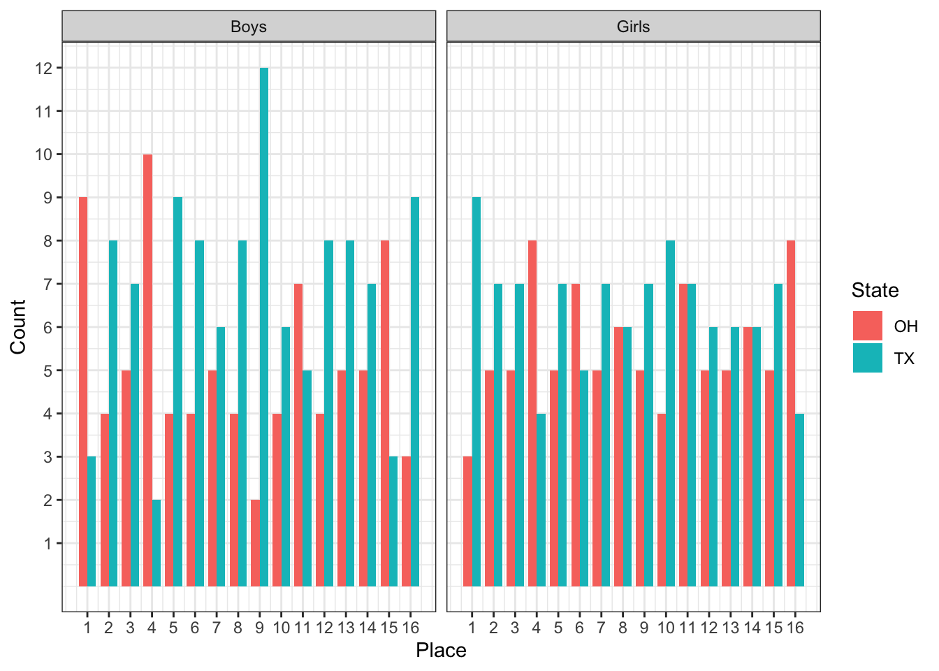

---

Swimmers of the Meet

Now for the awards. We’ll look for athletes who won two events (I keep saying, winning really is nice), and use the All-American standards as a tie-breaker.

Cuts_Link <-
  "https://raw.githubusercontent.com/gpilgrim2670/Pilgrim_Data/master/State_Cuts.csv"
Cuts <- read.csv(url(Cuts_Link))

'%!in%' <- function(x, y)
  ! ('%in%'(x, y)) # "not in" function

Cuts <- Cuts %>% # clean up Cuts
  filter(Stroke %!in% c("MR", "FR", "11 Dives")) %>%
  rename(Gender = Sex) %>%
  mutate(
    Event = case_when((Distance == 200 & #match events
                         Stroke == 'Free') ~ "200 Yard Freestyle",
                      (Distance == 200 &
                         Stroke == 'IM') ~ "200 Yard IM",
                      (Distance == 50 &
                         Stroke == 'Free') ~ "50 Yard Freestyle",
                      (Distance == 100 &
                         Stroke == 'Fly') ~ "100 Yard Butterfly",
                      (Distance == 100 &
                         Stroke == 'Free') ~ "100 Yard Freestyle",
                      (Distance == 500 &
                         Stroke == 'Free') ~ "500 Yard Freestyle",
                      (Distance == 100 &
                         Stroke == 'Back') ~ "100 Yard Backstroke",
                      (Distance == 100 &
                         Stroke == 'Breast') ~ "100 Yard Breaststroke",
                      TRUE ~ paste(Distance, "Yard", Stroke, sep = " ")
    ),
    
    Event = case_when(
      Gender == "M" ~ paste("Boys", Event, sep = " "),
      Gender == "F" ~ paste("Girls", Event, sep = " ")
    )
  )

Ind_Swimming_Results <- Results_Final %>%
  filter(str_detect(Event, "Diving|Relay") == FALSE) %>% # join Ind_Swimming_Results and Cuts
  left_join(Cuts %>% filter((Gender == "M" &
                               Year == 2020) |
                              (Gender == "F" &
                                 Year == 2019)) %>%
              select(AAC_Cut, AA_Cut, Event),
            by = 'Event')

Swimmer_Of_Meet <- Ind_Swimming_Results %>%
  mutate(
    AA_Diff = (Finals_Time_sec - sec_format(AA_Cut)) / sec_format(AA_Cut),
    Name = str_to_title(Name)
  ) %>%
  group_by(Name) %>%
  filter(n() == 2) %>% # get swimmers that competed in two events
  summarise(
    Avg_Place = sum(Place) / 2,
    AA_Diff_Avg = round(mean(AA_Diff, na.rm = TRUE), 3),
    Gender = unique(Gender),
    State = unique(State)
  ) %>%
  arrange(Avg_Place, AA_Diff_Avg) %>%
  group_split(Gender) # split out a dataframe for boys (1) and girls (2)

---

Boys

Swimmer_Of_Meet[[1]] %>%
  slice_head(n = 5) %>%
  select(-Gender) %>%
  ungroup() %>%
  flextable() %>%
  bold(part = "header") %>%
  bg(bg = "#D3D3D3", part = "header") %>%
  autofit()

---

Adam Chaney of Ohio won both sprint freestyle events and is your boys swimmer of the meet. Aaron Sequeira was actually slightly stronger on the All-American metric, but again, winning is important.

Results_Final %>%
  filter(Name == "Adam Chaney") %>%
  select(Place, Name, Team, Finals_Time, Event) %>%
  arrange(desc(Event)) %>%
  ungroup() %>%
  flextable() %>%
  bold(part = "header") %>%
  bg(bg = "#D3D3D3", part = "header") %>%
  autofit()

---

Girls

Swimmer_Of_Meet[[2]] %>%
  slice_head(n = 5) %>%
  select(-Gender) %>%
  ungroup() %>%
  flextable() %>%
  bold(part = "header") %>%
  bg(bg = "#D3D3D3", part = "header") %>%
  autofit()

---

Lillie Nordmann of Texas is your girls swimmer of the meet, winning two events and dominating the All-American metric. She’ll be swimming at Stanford next year. Lillie, (or other Cardinal swimmers) if you’re reading this, I’m confused. I get that Stanford is a great school and all, and I’m sure you’ll get a fantastic education going there. The swim teams are obviously massively successful, with great coaches, and with their help you’ll likely excel in the sport. I used to live in the Bay Area though, and it’s kind of cold there during the winter. Especially in the morning. Not cold like it is in New York, where I live now, but colder than I like it to be if I’m swimming outdoors. Stanford’s pool area is very nice, but it’s outdoors, no roof or anything. You’re signing up for four years of chilly mornings. It just doesn’t sound that good. I’m not against Stanford (or Cal - same situation) it’s just that there are good schools, with good swim teams, that have outdoor pools, but that are also in warm places. Or there are good schools with good swim teams in cold places but that have indoor pools. Either seems preferable to me. Just write in Lillie, let me know what I’m missing.

Kit Kat Zenick also won two events. She also apparently decided she likes the state of Ohio, because she’s headed back, to swim for Ohio State. Was it this meet that gave her such a favorable impression of the Buckeye State? Probably not since a) she committed before the meet was held and b) the meet is made up, only happening in our collective imaginations. Ohio State has a lovely, indoor, pool though, so I get it.

Results_Final %>%
  filter(Name == "Lillie Nordmann") %>%
  select(Place, Name, Team, Finals_Time, Event) %>%
  arrange(desc(Event)) %>%
  ungroup() %>%
  flextable() %>%
  bold(part = "header") %>%
  bg(bg = "#D3D3D3", part = "header") %>%
  autofit()

---

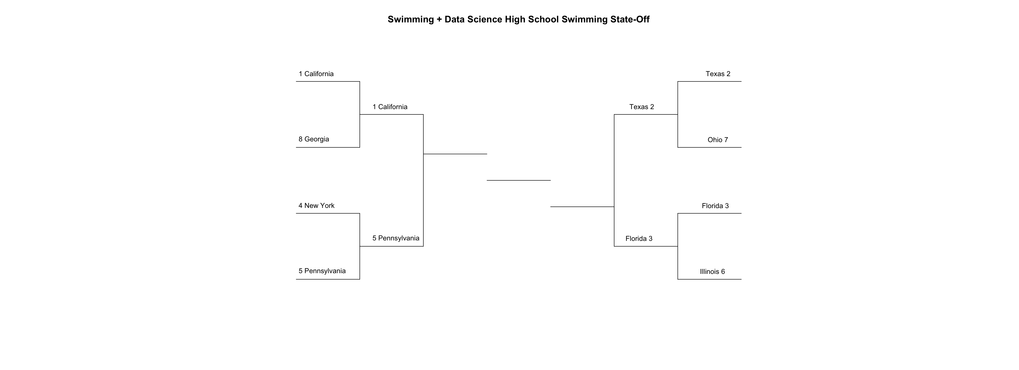
In Closing

This ends the first round of the High School Swimming State-Off Tournament, and that means it’s time to update our bracket. In March Madness the round of four is called the ‘Final Four’, which is odd since they redo it every year. I’m going to call mine the Fabulous Four, because if I do this again next year, there’ll just be more fabulousness, and that’s fine by me.

draw_bracket(
  teams = c(
    "California",
    "Texas",
    "Florida",
    "New York",
    "Pennsylvania",
    "Illinois",
    "Ohio",
    "Georgia"
  ),
  round_two = c("California", "Texas", "Florida", "Pennsylvania"),
  title = "Swimming + Data Science High School Swimming State-Off",
  text_size = 0.9
)