In a previous post we discussed the 2020 USMS ePostal results, and hypothesized that declines in average distances swum by older age groups are caused by higher proportions of weaker swimmers participating in older age groups, rather than age based declines. We also mentioned how USMS ePostal results are observational data, and so we can’t draw any strict causal relationships. What we can do though is idly speculate, and that’s pretty fun too.

USMS has published results from the ePostal dating back to 1998, but in decidedly unfriendly formats. However, driven by an excess of COVID 19 enforced free time my love of swimming I’ve cleaned them all up and made them available tidy-style. Let’s load some packages and grab that data.

library(readr)
library(dplyr)
library(tidyr)
library(ggplot2)

urlfile <- "https://raw.githubusercontent.com/gpilgrim2670/Pilgrim_Data/master/Postal_All.csv"
df_all <- read_csv(url(urlfile))

I cleaned the ePostal data with the idea of just poking at it to see if anything interesting came out. First step is just to plot the total number of participants for each year.

df_all %>% 
  group_by(Year, Gender) %>% 
  summarise(Count = n()) %>% 
  arrange(desc(Count)) %>% 
  ggplot(aes(x = Year, y = Count)) +
  geom_line(aes(color = Gender)) +
  geom_point(aes(color = Gender)) +
  scale_x_continuous(breaks = seq(1998, 2020, 2)) +
  theme_bw() +
  theme(axis.text.x = element_text(angle = 45, hjust = 1)) +
  labs(y = "Total No. Swimmers",
       title = "USMS ePostal Participation vs. Year")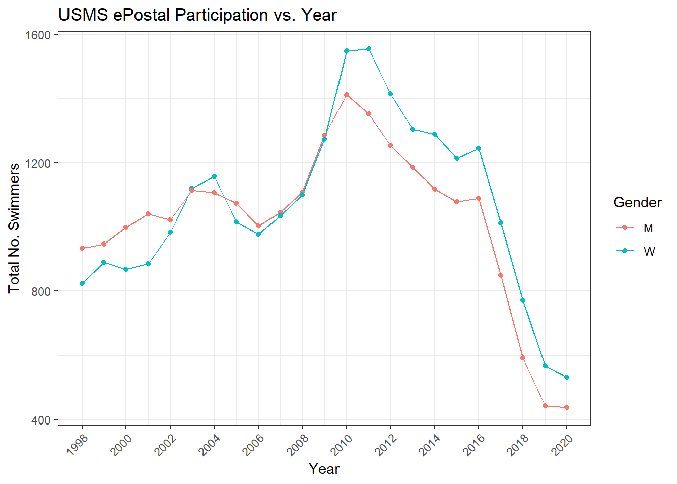

There are some features worth taking a look at. Namely the huge jump in years 2008-2011 and then the precipitous decline beginning in 2017. Let’s start with the big jump. One possible explanation is the Olympics. They’re the biggest, highest profile swim meet on the planet, and in 2008 they were all the more so, because the 2008 Beijing Games were where Michael Phelps won 8 gold medals. It was awesome and loads of Americans watched. Myabe some swimmers hit the next year’s ePostal a bit more motivated. Note: ePostals are contested in the January-March time frame (exact dates vary by year), so the next ePostal after the 2008 games was in 2009.

df_all %>% 
  group_by(Year, Gender) %>% 
  summarise(Count = n()) %>% 
  arrange(desc(Count)) %>% 
  ggplot(aes(x = Year, y = Count)) +
  geom_line(aes(color = Gender)) +
  geom_point(aes(color = Gender), size = 2.5) +
  scale_x_continuous(breaks = seq(1998, 2020, 2)) +
  theme_bw() +
  theme(axis.text.x = element_text(angle = 45, hjust = 1)) +
  labs(y = "Total No. Swimmers",
       title = "USMS ePostal Participation vs. Year") +
  geom_vline(xintercept = 2001, linetype = 2) +
  annotate("label", x = 2001, y = 1150, label = "Olympics") +
  geom_vline(xintercept = 2005, linetype = 2) +
  annotate("label", x = 2005, y = 1250, label = "Olympics") +
  geom_vline(xintercept = 2009, linetype = 2) +
  annotate("label", x = 2009, y = 1650, label = "Phelps 8x Golds!") +
  geom_vline(xintercept = 2013, linetype = 2) +
  annotate("label", x = 2013, y = 1530, label = "Olympics") +
  geom_vline(xintercept = 2017, linetype = 2) +
  annotate("label", x = 2017, y = 1325, label = "Olympics")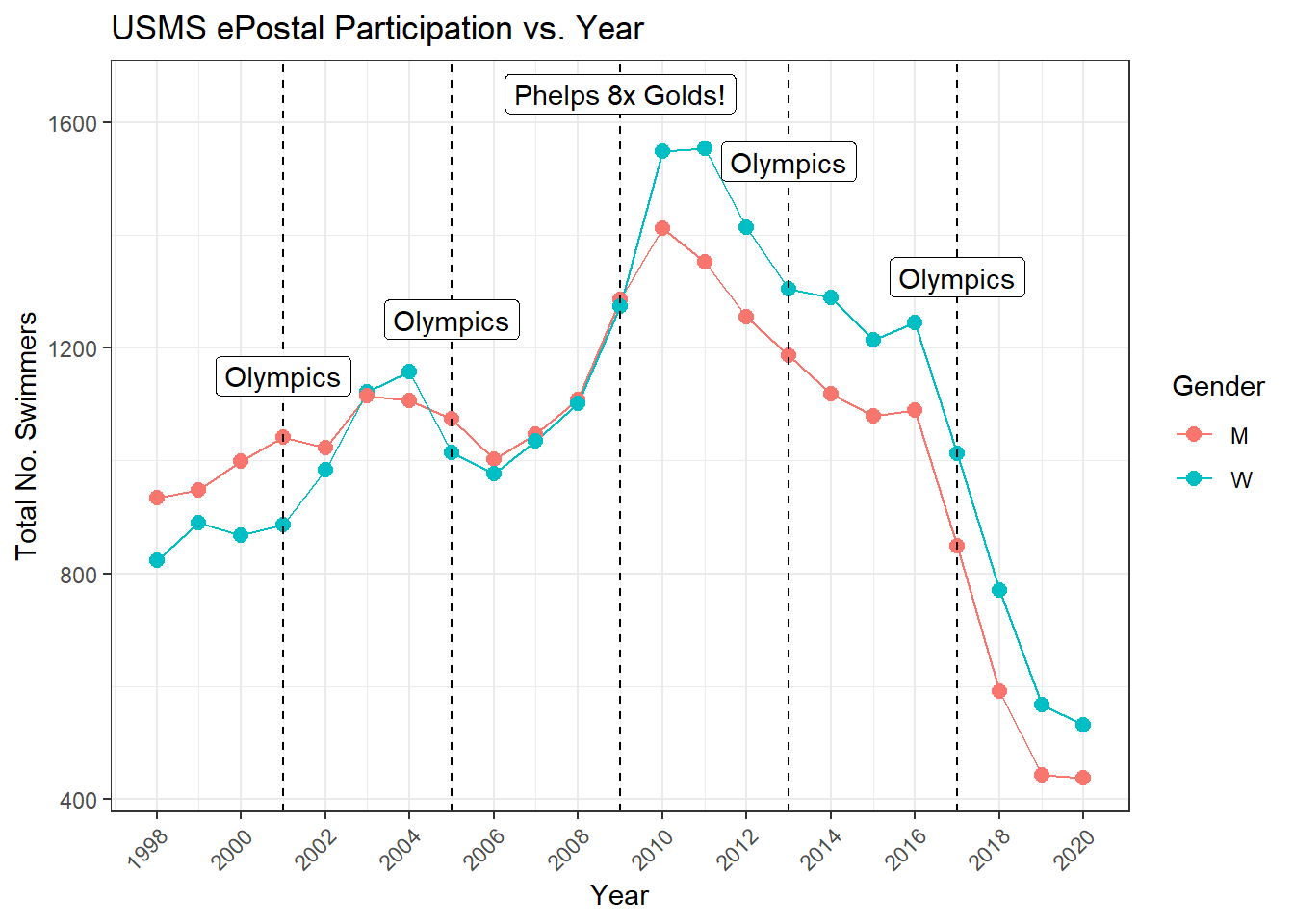

So maybe there are Olympics bumps, but maybe not. With all due respect to Mr. Phelps, the greatest swimmer of all time, I’d like to propose an alternative explanation for the huge surge in ePostal participation between 2008 and 2011. It’s simple, we kill dress like the Batman.

The 2008 Games saw the rise of so-called “Super Suits”, beginning with the Speedo LZR, and eventually including fully rubberized options by Blue Seventy, Arena, and many others. People loved them, but almost immediately there was talk of banning them. When I say people loved them, Masters swimmers particularly loved them, and USMS was the last organization to ban them, effective May 22, 2010. The suits were exciting, they were fast, and for men with a bit of gut, they helped with that as well!

That’s my theory - a heady mixture of Phelpsian excellence and sleek sexy polyurethane caused a spike in ePostal participation. Can’t say for sure, but that’s what I’m going with.

To explain the decline beginning in 2017 I thought I’d take a look at participation by age group. Originally I used facet_grid to facet by age group, but then I thought about one of those fancy animated internet plots that moves with time. This is the internet, and for all you dear readers know I’m a fancy internet expert. So here’s my fancy plot.

library(gganimate)
p <- df_all %>% 
  filter(is.na(Age) == FALSE) %>% 
  ggplot(aes(x = Age_Group)) +
  geom_bar(aes(fill = Gender), position = "dodge") +
  theme_bw() +
  theme(axis.text.x = element_text(angle = 45, hjust = 1)) +
  transition_time(Year) +
  labs(title = "Year: {round(frame_time, 0)}",
       x = "Age Group",
       y = "No. Participants")
animate(p, fps = 5)

What we see is that overall numbers go down, and that participation shifts older. USMS released membership trend data through August 2018, showing fraction of total membership by age group.

urlfile_2 <- "https://raw.githubusercontent.com/gpilgrim2670/Pilgrim_Data/master/USMS_Membership_Trends.csv"
Membership_Trends <- read_csv(url(urlfile_2))

Membership_Trends_Long <- Membership_Trends %>% 
  pivot_longer(cols = -Age_Group, names_to = "Year", values_to = "Count") %>% 
  group_by(Year) %>% 
  mutate(Year_Total = sum(Count)) %>% 
  group_by(Age_Group) %>% 
  mutate(Percent = Count/Year_Total * 100)

Plotting membership fraction by year shows the baby boomer wave passing through. The Boomers are approximately in their 50s in 2017, so still of prime age to be participating in the ePostal.

'%!in%' <- function(x,y)!('%in%'(x,y))

Membership_Trends_Long %>% 
  filter(Age_Group %!in% c("80-84", "85-89", "90-94", "95-99", "100-104", "105+")) %>% 
  ggplot(aes(x = as.numeric(Year), y = Percent)) +
  geom_point(aes(color = Age_Group)) +
  geom_line(aes(color = Age_Group)) +
  scale_x_continuous(breaks = seq(1985, 2020, 5)) +
  scale_y_continuous(breaks = seq(0, 25, 5)) +
  coord_cartesian(ylim = c(0, 22)) +
  theme_bw() +
  labs(x = "Year",
      y = "% of Total USMS Membership",
      color = "Age Group",
      title = "USMS Age Group Percentage by Year")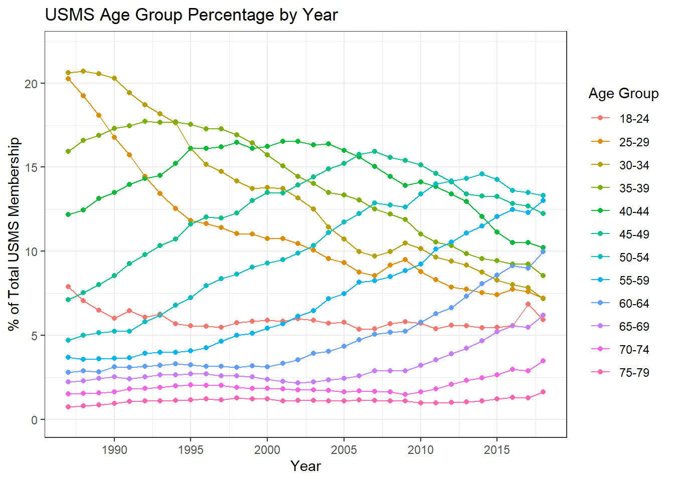

Membership_Trends_Long %>% 
  group_by(Year) %>% 
  filter(Percent == max(Percent)) %>% 
  ggplot(aes(x = as.numeric(Year), y = Percent)) +
  geom_point(aes(color = Age_Group)) +
  geom_line(aes(color = Age_Group)) +
  scale_x_continuous(breaks = seq(1985, 2020, 5)) +
  scale_y_continuous(breaks = seq(0, 25, 5)) +
  # viridis::scale_color_viridis(discrete = TRUE) +
  coord_cartesian(ylim = c(0, 22)) +
  theme_bw() +
  labs(x = "Year",
       y = "% of Total USMS Membership",
       color = "Age Group",
       title = "Largest USMS Age Group by Year")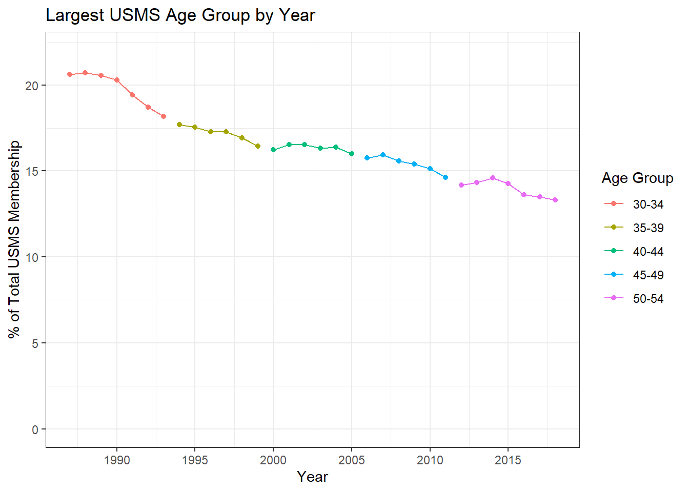

Looking at the average distance swam by each swimmer per year shows something interesting.

df_all %>% 
  group_by(Year, Gender) %>% 
  summarise(Avg_Distance = mean(Distance, na.rm = TRUE)) %>% 
  ggplot(aes(x = Year, y = Avg_Distance)) +
  geom_point(aes(color = Gender)) +
  geom_line(aes(color = Gender)) +
  scale_x_continuous(breaks = seq(1998, 2020, 2)) +
  theme_bw() +
  labs(y = "Average Distance",
       title = "USMS ePostal Average Distance Covered by Year")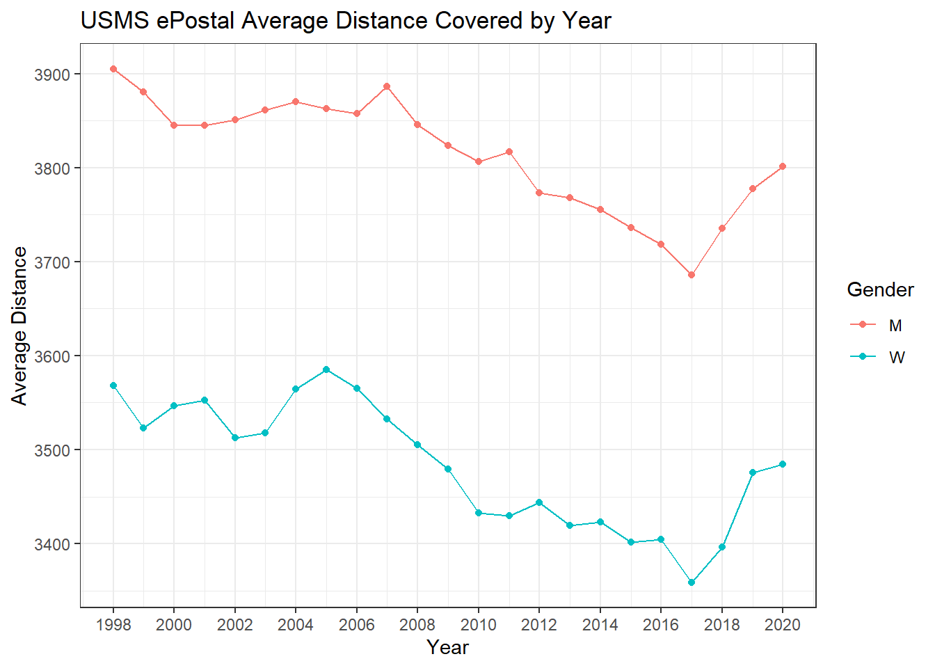

Average distance had been declining every year, which matches with the slowly aging USMS membership population.

In 2017 though average distance shoots up, meaning that while fewer swimmers are reporting their results, those that do are swimming further.

A sharp change like this makes me suspect that rather than some gradual cause, like aging, there must have been some distinct event. It turns out that in 2017, per the advice of legal council, USMS disallowed group submission of ePostal results. What this means practically is that in the years before 2017 a swim club would organize a postal event for its membership. They’d get pool time, have athletes come down and swim, as well as count for each other, using official counter sheets. The club would then collect those counter sheets, and with each athlete’s permission, submit the results. Lots of results got submitted, because the barrier to doing so was quite low - the club handled it. Now each athlete has to take their individual results home and remember to submit them - voila! fewer people do so. It makes sense that those athletes who are invested enough to submit their results would also be faster than those who are not.

Updated: 18 November, 2021
Created: 12 May, 2020