Tokyo 2020 Olympic Results

Omega, the official timing partner of the Olympics, has released swimming results by round (heats, semis, finals) and event. That’s a lot of pdf files, but I’ve collected them into a Github repository here. We can use SwimmeR to parse all of them and build a single data frame with all the 2020 Olympic results. Collecting and parsing the results will proceed in much the same way as other Swimming + Data Science adventures like Scraping Websites and Building a Large Dataset with SwimmeR, Dataset of All ISL Results Season 1 and 2 and COVID Impacts in Swimming Results?.

Basically assemble a list of links with tools from the rvest package and then map SwimmeR’s read_results followed by swim_parse over that list.

Here’s the list of links, nicely cleaned up.

tokyo_url <- "https://github.com/gpilgrim2670/Pilgrim_Data/tree/master/Tokyo2020" # repository url
selector <- ".js-navigation-open" # selector where links are kept
page_contents <- read_html(tokyo_url) # get content of repository web page
tokyo_links <- html_attr(html_nodes(page_contents, selector), "href") # raw links extracted from selector node

tokyo_links <- paste0("https://github.com", tokyo_links) # add beginning to link
tokyo_links <- str_replace(tokyo_links, "blob", "raw") # replace blob with raw
tokyo_links <- tokyo_links[6:95] # only want links 7-19, the rest aren't swimming results
tokyo_links <- tokyo_links[is.na(tokyo_links) == FALSE] # don't want NA links
tokyo_links <- tokyo_links[str_detect(tokyo_links, "\\.rds") == FALSE] # don't want the .rds file of compiled results
head(tokyo_links) # print a few links

And here’s the mapping of read_results and swim_parse.

tokyo <- map(tokyo_links, safely(read_results, otherwise = NA)) # read_results with safely to keep going even if there are errors.  No errors are expected.
tokyo <- SwimmeR::discard_errors(tokyo) # discard errors (there aren't actually any)

tokyo_parse <- map(tokyo, safely(swim_parse, otherwise = NA), splits = TRUE, relay_swimmers = TRUE) # swim_parse with safely to parse results
tokyo_parse <- SwimmeR::discard_errors(tokyo_parse) # discard errors (there aren't actually any)

tokyo_df <- bind_rows(tokyo_parse) # bind into data frame

Ta-da! Here’s the final of the Men’s 100 Fly just to show off what we’ve got.

tokyo_df %>% 
  filter(Event == "Men's 100m Butterfly",
         Heat == "Final") %>% 
  select(where(~ !(all(is.na(.)))),
         -Heat) %>% 
  relocate(any_of(c("DQ", "Exhibition")), .after = last_col()) %>% 
  flextable_style()

Reaction Times and Volleyball

Years ago there was an event called the Empire State Games. It was an Olympics style event held in New York every year, with winter and summer versions hosted at different SUNY campuses across the state. It was awesome but sadly is no more, a victim of budget cuts.

One year when I was competing the Games were held at SUNY Binghamton. SUNY Binghamton doesn’t have a 50m pool though, so the swimming portion was actually held 90 minutes away at SUNY Cortland. For other reasons unknown to me volleyball was also held at SUNY Cortland, which meant I watched a lot of volleyball. I’d never really seen volleyball before, and found it to be very enjoyable. I enjoyed women’s volleyball more than men’s but wasn’t really sure why (it wasn’t the shorts, don’t be disrespectful).

After puzzling on it for the entire week I came up with this theory.

1. The most exciting thing in volleyball are the volleys, where the ball goes back and forth a lot
   • The longer the volley the more exciting it is
2. The men’s volleyball game has higher powered offense than the women’s game
   • Male volleyball players are on average taller and stronger than female volleyball players
   • Male players spike the ball down at sharper angles on average, because they’re taller
   • Male players hit the ball faster on average, because they’re stronger
3. Defense is largely driven by ability to see a ball coming in and react to block/dig/save it
   • Reaction time matters most
   • There probably aren’t gendered differences in reaction time

Summing up - the women’s volleyball game has relatively stronger defense vs. offense, leading to longer volleys and a more exciting game

It was over a decade ago that I came up with my theory, and now is the time to test it. Those Tokyo Olympic swimming results have reaction times, and while swimmers aren’t volleyball players I think there’s reason to believe that gender differences in reaction time, if they even exist, will hold across sports.

tokyo_df_gender <- tokyo_df %>% 
  filter(str_detect(Event, "Relay") == FALSE) %>% 
  mutate(Gender = case_when(str_detect(Event, "Men") ~ "M",
                            str_detect(Event, "Women") ~ "F"))

Here’s the Women’s 100 Fly, with a Gender column.

tokyo_df_gender %>% 
  filter(Event == "Women's 100m Butterfly",
         Heat == "Final") %>% 
  select(where(~ !(all(is.na(.)))),
         -Heat) %>% 
  relocate(any_of(c("DQ", "Exhibition")), .after = last_col()) %>% 
  flextable_style()

Now all we need to do is collect reaction times by athlete and then by gender.

tokyo_df_gender %>% 
  group_by(Name) %>% 
  summarise(Reaction_Time_Avg = mean(as.numeric(Reaction_Time), na.rm = TRUE),
            Team = unique(Team)) %>% 
  arrange(Reaction_Time_Avg) %>% 
  head(5) %>% 
  flextable_style()

Hmmm, something interesting has happened. You may not know it, but all of those athletes are backstrokers. Backstroke uses a different start compared to the other swimming disciplines, so we need to address that.

tokyo_df_gender <- tokyo_df_gender %>% 
  group_by(Name, Event) %>% 
  summarise(Reaction_Time_Avg = mean(as.numeric(Reaction_Time), na.rm = TRUE),
            Team = unique(Team),
            Gender = unique(Gender)) %>%
  mutate(Discipline = case_when(str_detect(Event, "Back") ~ "Backstroke",
                                TRUE ~ "Not Backstroke")) %>% 
  filter(Reaction_Time_Avg < 1)

tokyo_df_gender %>% 
  ggplot() +
  geom_histogram(aes(x = Reaction_Time_Avg, fill = Discipline), position = "identity", alpha = 0.5) +
  theme_bw() +
  labs(title = "Reaction Time Differences by Start Type",
       y = "Number of Athletes",
       x = "Average Reaction Time (s)")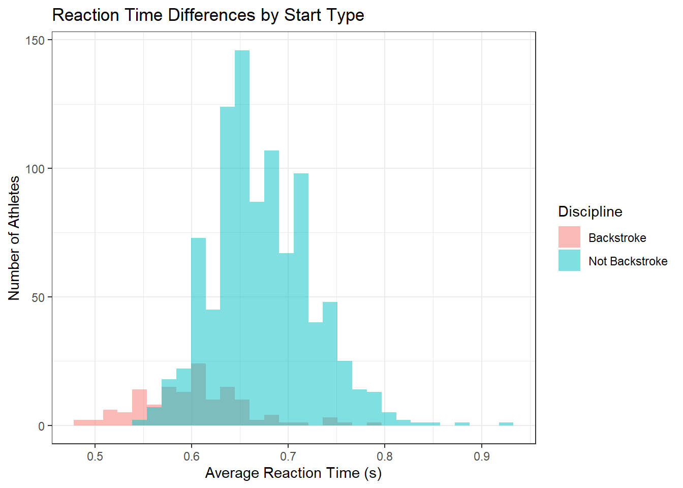

Breaking gender out visually - looks about the same to me. We’ll need to test to be sure though.

tokyo_df_gender %>% 
  ggplot() +
  geom_histogram(aes(x = Reaction_Time_Avg, fill = Discipline), position="identity", alpha = 0.5) +
  theme_bw() +
  facet_wrap(. ~ Gender) +
  labs(title = "Reaction Time Differences by Gender and Start Type",
       y = "Number of Athletes",
       x = "Average Reaction Time (s)")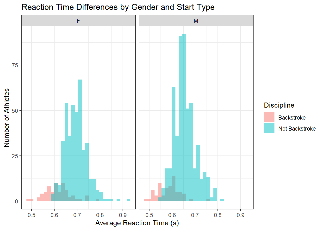

T Tests for Comparison

Histogram data looks normally distributed, so t tests are appropriate means of comparing two sets of data. Throughout I’ll use 0.01 (99%) as my significance level.

female_backstrokers <- tokyo_df_gender %>% 
  filter(Gender == "F",
         Discipline == "Backstroke")

male_backstrokers <- tokyo_df_gender %>% 
  filter(Gender == "M",
         Discipline == "Backstroke")

female_nonbackstrokers <- tokyo_df_gender %>% 
  filter(Gender == "F",
         Discipline == "Not Backstroke")

male_nonbackstrokers <- tokyo_df_gender %>% 
  filter(Gender == "M",
         Discipline == "Not Backstroke")

all_backstrokers <- tokyo_df_gender %>% 
  filter(Discipline == "Backstroke")

all_nonbackstrokers <- tokyo_df_gender %>% 
  filter(Discipline == "Not Backstroke")

back_t.test <- t.test(female_backstrokers$Reaction_Time_Avg, male_backstrokers$Reaction_Time_Avg)
back_t.test

## 
##  Welch Two Sample t-test
## 
## data:  female_backstrokers$Reaction_Time_Avg and male_backstrokers$Reaction_Time_Avg
## t = 3.2722, df = 129.01, p-value = 0.001369
## alternative hypothesis: true difference in means is not equal to 0
## 95 percent confidence interval:
##  0.01177603 0.04779629
## sample estimates:
## mean of x mean of y 
## 0.6152451 0.5854589

non_back_t.test <- t.test(female_nonbackstrokers$Reaction_Time_Avg, male_nonbackstrokers$Reaction_Time_Avg)
non_back_t.test

## 
##  Welch Two Sample t-test
## 
## data:  female_nonbackstrokers$Reaction_Time_Avg and male_nonbackstrokers$Reaction_Time_Avg
## t = 12.711, df = 890.73, p-value < 2.2e-16
## alternative hypothesis: true difference in means is not equal to 0
## 95 percent confidence interval:
##  0.03393902 0.04633348
## sample estimates:
## mean of x mean of y 
## 0.6956908 0.6555545

back_non_back_t.test <- t.test(all_backstrokers$Reaction_Time_Avg, all_nonbackstrokers$Reaction_Time_Avg)
back_non_back_t.test

## 
##  Welch Two Sample t-test
## 
## data:  all_backstrokers$Reaction_Time_Avg and all_nonbackstrokers$Reaction_Time_Avg
## t = -14.579, df = 173.18, p-value < 2.2e-16
## alternative hypothesis: true difference in means is not equal to 0
## 95 percent confidence interval:
##  -0.08276967 -0.06303023
## sample estimates:
## mean of x mean of y 
## 0.6002433 0.6731433

reaction_time_gender <- tokyo_df_gender %>% 
  ungroup() %>% 
  group_by(Gender, Discipline) %>% 
  summarise(Reaction_Time_Avg_2 = mean(Reaction_Time_Avg, na.rm = TRUE)) %>% 
  ungroup() %>% 
  group_split(Discipline)

reaction_time_backstroke <- tokyo_df_gender %>% 
  ungroup() %>% 
  group_by(Gender, Discipline) %>% 
  summarise(Reaction_Time_Avg_2 = mean(Reaction_Time_Avg, na.rm = TRUE)) %>% 
  ungroup() %>% 
  group_split(Gender)

My Volleybal Theory Revisited

So we’re seeing a statistically significant difference between the reaction times of male and female swimmers. That said, what’s the actual difference?

tokyo_df_gender %>% 
  group_by(Gender, Discipline) %>% 
  summarise(Reaction_Time_Avg = round(mean(Reaction_Time_Avg, na.rm = TRUE), 2)) %>% 
  arrange(Discipline) %>% 
  flextable_style()

## `summarise()` has grouped output by 'Gender'. You can override using the `.groups` argument.

The differences between men and women are a few hundreths of a second in reaction time, or about 5%. It’s something, sometimes the difference between a gold and a silver medal. The question with respect to my volleyball theory though is how does that difference in reaction times compare to the differences in ball velocity when hit by men vs. women.

There’s lots of sports science about ball velocity in volleyball. This review article¹ collects much of it and cites this article² reporting the spike speeds of elite male Italian players using an elevation style spike at 25.6 m/s and similarly elite female Italian players spiking the ball at 20.1 m/s using the elevation style. Comparable numbers are observed for athletes using the backswing style of spike. That means men spike approximately 25% faster than women. We found men’s reaction times to only be about 5% faster than women’s. From the evidence I’ve been able to uncover so far I’m concluding that my theory is largely correct. The women’s volleyball games I observed probably did have longer volleys. Of course if I’d been really on my game I would have counted some, but that ship has sailed. This analysis could also be deepened, perhaps by including a race-type component when considering swimmer reaction times.

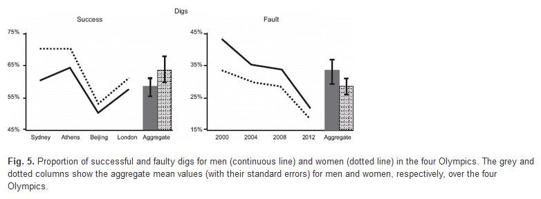
There is also some literature evidence for my theory - that defense is relatively more potent compared to offense in women’s volleyball than in men’s volleyball. Here³ authors show that women have more successful digs, and fewer faulty digs than men at the 2000, 2004, 2008 and 2016 Olympics.

In Closing

The key messages I hope you’ll take from investigating my volleyball theory have nothing to do with gender based performance differences. Instead they are:

1. Domain specific knowledge is important. Recognizing differences between backstroke starts and the forward starts used in other events requires knowledge not just of R or stats, but of the actual topic at hand - swimming
2. Just because a t-test tells you that there’s a statistically significant difference between two populations doesn’t mean the difference actually matters in your evaluation. A 5% difference in reaction times is dwarfed by a 25% difference in ball speed
3. SwimmeR is an awesome package and you should tell all your friends about it

Thanks for reading, we hope to see you again here at [Swimming + Data Science]!

References

1. Oliveira L dos S, Moura TBMA, Rodacki ALF, Tilp M, Okazaki VHA. A systematic review of volleyball spike kinematics: Implications for practice and research. International Journal of Sports Science & Coaching. 2020;15(2):239-255. doi:10.1177/1747954119899881

2. Seminati E, Marzari A, Vacondio O, et al. Shoulder 3D range of motion and humerus rotation in two volleyball spike techniques: injury prevention and performance. Sports Biomech 2015; 14: 216–231

3. Kountouris P, Drikos S, Aggelonidis I, Laios A, Kyprianou M. Evidence for Differences in Men’s and Women’s Volleyball Games Based on Skills Effectiveness in Four Consecutive Olympic Tournaments. Comprehensive Psychology. January 2015. doi:10.2466/30.50.CP.4.9