High School Swimming State-Off Tournament California (1) vs. Pennsylvania (5)
Here we have it, the last meet of the State-Off semi-final round, where California (1) takes on the Cinderella story that is Pennsylvania (5) for a trip to the finals. Don’t forget to update your version of SwimmeR to 0.4.1, because we’ll be using some newly released functions. We’ll also do some more plotting/data-vis and use prop.test to do some statistical work with the results, this time looking at grade distributions across events.
library(SwimmeR)
library(dplyr)
library(purrr)
library(tidyr)
library(stringr)
library(flextable)
library(ggplot2)
Please note the following analysis was updated November 22nd 2020 to reflect changes beginning with SwimmeR v0.6.0 released via CRAN on November 22nd 2020. Please make sure your version of SwimmeR is up-to-date.
My flextable styling function is still working great since I made it last week so why mess with a good thing? Here it is again.
flextable_style <- function(x) {
  x %>%
    flextable() %>%
    bold(part = "header") %>% # bolds header
    bg(bg = "#D3D3D3", part = "header") %>% # puts gray background behind the header row
    autofit()
}
Getting Results
As discussed previously we’ll just grab clean results that I’m hosting on github rather than going through the exercise of reimporting them with SwimmeR.
California_Link <-
  "https://raw.githubusercontent.com/gpilgrim2670/Pilgrim_Data/master/CA_States_2019.csv"
California_Results <- read.csv(url(California_Link)) %>%
  mutate(State = "CA")
Pennsylvania_Link <-
"https://raw.githubusercontent.com/gpilgrim2670/Pilgrim_Data/master/PA_States_2020.csv"
Pennsylvania_Results <- read.csv(url(Pennsylvania_Link)) %>%
mutate(State = "PA")Results <- California_Results %>%
bind_rows(Pennsylvania_Results) %>%
mutate(Gender = case_when(
str_detect(Event, "Girls") == TRUE ~ "Girls",
str_detect(Event, "Boys") == TRUE ~ "Boys"
)) %>%
filter(str_detect(Event, "Swim-off") == FALSE) %>%
rename("Team" = School,
"Age" = Grade)
Scoring the Meet
Results_Final <- results_score(
  results = Results,
  events = unique(Results$Event),
  meet_type = "timed_finals",
  lanes = 8,
  scoring_heats = 2,
  point_values = c(20, 17, 16, 15, 14, 13, 12, 11, 9, 7, 6, 5, 4, 3, 2, 1)
)

Scores <- Results_Final %>%
  group_by(State, Gender) %>%
  summarise(Score = sum(Points))

Scores %>%
  arrange(Gender, desc(Score)) %>%
  ungroup() %>%
flextable_style()State | Gender | Score |
CA | Boys | 1,641 |
PA | Boys | 684 |
CA | Girls | 1,629 |
PA | Girls | 696 |
Scores %>%
  group_by(State) %>%
  summarise(Score = sum(Score)) %>%
  arrange(desc(Score)) %>%
  ungroup() %>%
flextable_style()State | Score |
CA | 3,270 |
PA | 1,380 |
Pennsylvania’s charmed run through (one round of) the State-Off Tournament has come to an end, with California dominating both the boys and girls meets, and winning the overall handily.
Swimmers of the Meet
Swimmer of the Meet criteria is the same as it’s been for the entire State-Off. First we’ll look for athletes who have won two events, thereby scoring a the maximum possible forty points. In the event of a tie, where multiple athletes win two events, we’ll use All-American standards as a tiebreaker. Will anyone join Lillie Nordmann as a multiple Swimmer of the Meet winner?
Cuts_Link <-
  "https://raw.githubusercontent.com/gpilgrim2670/Pilgrim_Data/master/State_Cuts.csv"
Cuts <- read.csv(url(Cuts_Link))

Cuts <- Cuts %>% # clean up Cuts
  filter(Stroke %!in% c("MR", "FR", "11 Dives")) %>% # %!in% is now included in SwimmeR
  rename(Gender = Sex) %>%
  mutate(
    Event = case_when((Distance == 200 & #match events
                         Stroke == 'Free') ~ "200 Yard Freestyle",
                      (Distance == 200 &
                         Stroke == 'IM') ~ "200 Yard IM",
                      (Distance == 50 &
                         Stroke == 'Free') ~ "50 Yard Freestyle",
                      (Distance == 100 &
                         Stroke == 'Fly') ~ "100 Yard Butterfly",
                      (Distance == 100 &
                         Stroke == 'Free') ~ "100 Yard Freestyle",
                      (Distance == 500 &
                         Stroke == 'Free') ~ "500 Yard Freestyle",
                      (Distance == 100 &
                         Stroke == 'Back') ~ "100 Yard Backstroke",
                      (Distance == 100 &
                         Stroke == 'Breast') ~ "100 Yard Breaststroke",
                      TRUE ~ paste(Distance, "Yard", Stroke, sep = " ")
    ),

    Event = case_when(
      Gender == "M" ~ paste("Boys", Event, sep = " "),
      Gender == "F" ~ paste("Girls", Event, sep = " ")
    )
  )

Ind_Swimming_Results <- Results_Final %>%
  filter(str_detect(Event, "Diving|Relay") == FALSE) %>% # join Ind_Swimming_Results and Cuts
  left_join(Cuts %>% filter((Gender == "M" &
                               Year == 2020) |
                              (Gender == "F" &
                                 Year == 2019)) %>%
              select(AAC_Cut, AA_Cut, Event),
            by = 'Event')

Swimmer_Of_Meet <- Ind_Swimming_Results %>%
  mutate(
    AA_Diff = (Finals_Time_sec - sec_format(AA_Cut)) / sec_format(AA_Cut),
    Name = str_to_title(Name)
  ) %>%
  group_by(Name) %>%
  filter(n() == 2) %>% # get swimmers that competed in two events
  summarise(
    Avg_Place = sum(Place) / 2,
    AA_Diff_Avg = round(mean(AA_Diff, na.rm = TRUE), 3),
    Gender = unique(Gender),
    State = unique(State)
  ) %>%
  arrange(Avg_Place, AA_Diff_Avg) %>%
  group_split(Gender) # split out a dataframe for boys (1) and girls (2)
Boys
Swimmer_Of_Meet[[1]] %>%
  slice_head(n = 5) %>%
  select(-Gender) %>%
  ungroup() %>%
flextable_style()Name | Avg_Place | AA_Diff_Avg | State |
Brownstead, Matt | 1.0 | -0.050 | PA |
Mefford, Colby | 1.5 | -0.027 | CA |
Hu, Ethan | 2.0 | -0.052 | CA |
Jensen, Matthew | 2.0 | -0.038 | PA |
Faikish, Sean | 2.0 | -0.032 | PA |
Turns out yes, Matt Brownstead from Pennsylvania joins Lillie in the multiple winners club. As we discussed previously Matt broke the national high school record in the 50 free, so that guaranteed him one win. He also won the 100 free - the only boy here to win two events. We don’t even need to go to the All-American tie breaker, but it is worth noting that Ethan Hu outperformed Matt by that metric. Pennsylvania also managed three of the top five finishers here - very nice!
Results_Final %>%
  filter(Name == "Brownstead, Matt") %>%
  select(Place, Name, Team, Finals_Time, Event) %>%
  arrange(desc(Event)) %>%
  ungroup() %>%
flextable_style()Place | Name | Team | Finals_Time | Event |
1 | Brownstead, Matt | State College-06 | 19.24 | Boys 50 Yard Freestyle |
1 | Brownstead, Matt | State College-06 | 43.29 | Boys 100 Yard Freestyle |
Girls
Swimmer_Of_Meet[[2]] %>%
  slice_head(n = 5) %>%
  select(-Gender) %>%
  ungroup() %>%
  flextable() %>%
  bold(part = "header") %>%
  bg(bg = "#D3D3D3", part = "header") %>%
autofit()Name | Avg_Place | AA_Diff_Avg | State |
Hartman, Zoie | 1.0 | -0.047 | CA |
Ristic, Ella | 1.0 | -0.023 | CA |
Tuggle, Claire | 1.5 | -0.031 | CA |
Delgado, Anicka | 1.5 | -0.023 | CA |
Kosturos, Sophi | 2.0 | -0.021 | CA |
Zoie Hartman heads a California sweep of the girls swimmer of the meet top 5 while also winning her second swimmer of the meet crown.
Results_Final %>%
  filter(Name == "Hartman, Zoie") %>%
  select(Place, Name, Team, Finals_Time, Event) %>%
  arrange(desc(Event)) %>%
  ungroup() %>%
flextable_style()Place | Name | Team | Finals_Time | Event |
1 | Hartman, Zoie | Monte Vista_NCS | 1:55.29 | Girls 200 Yard IM |
1 | Hartman, Zoie | Monte Vista_NCS | 59.92 | Girls 100 Yard Breaststroke |
Performances By Grade
It might be interesting to see what fraction of athletes from each grade compete in various events. We might hypothesize that sprint events, like the 50 freestyle in particular, would have a higher percentage of older athletes, who benefit from extra years of growth, muscle development etc. SwimmeR can capture grade (or age) values, assuming they’re present in the original results. In this case we do have grade values, so let’s take a look.
Results_Age <- Results_Final %>%
  filter(is.na(Age) == FALSE,
         Age %!in% c("ST", "1")) %>% # remove nonsense values
  mutate(
    Age = case_when(
      # regularize encoding of grade values
      Age == "9" ~ "FR",
      Age == "10" ~ "SO",
      Age == "11" ~ "JR",
      Age == "12" ~ "SR",
      TRUE ~ Age
    )
  ) %>%
  mutate(Age = factor(Age, levels = c("FR", "SO", "JR", "SR"))) %>% # factor to order grade levels
  filter(str_detect(Event, "Relay") == FALSE) %>% # remove relays since they don't have grades
  mutate(Event = str_remove(Event, "Girls |Boys "),
         Event = factor(Event, levels = rev(unique(
           # order events by meet order, in this case with diving first
           str_remove(unique(Results$Event), "Girls |Boys ")
         ))))

Results_Age_Sum <- Results_Age %>%
  group_by(Event, Gender, Age) %>%
  summarise(Numb = n()) %>% # number of athletes for each event/gender/grade combination
  ungroup() %>%
  group_by(Event, Gender) %>%
  mutate(Percentage = Numb / sum(Numb)) # percentage of athletes in each grade for each event/gender combination

Results_Age_Sum %>%
  ggplot() +
  geom_col(aes(x = Event, y = Percentage, fill = Age)) +
  coord_flip() +
  facet_wrap(. ~ Gender) +
  theme_bw() +
  labs(y = "Frequency")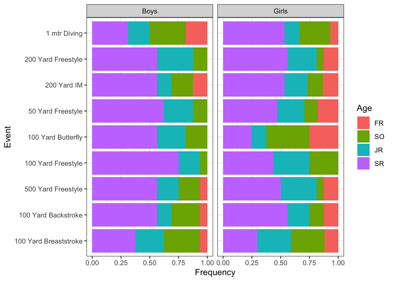
That’s a lovely plot (if I do say so myself). Interestingly, the 50 freestyle doesn’t appear to be the most senior heavy event for boys or girls. It would be nice though to have the data in a table form to aid in taking a closer look, so let’s work on that.
Tables
# Split results by gender, creating a list of two dataframes
Results_Age_Gender <- Results_Age_Sum %>%
  ungroup() %>%
  group_by(Gender) %>%
  group_split()

# function to apply to both dataframes that will produce columns with percentages for each grade and event
Age_Fill <- function(x) {
  x <- x %>%
    mutate(Percentage = round(Percentage, 2)) %>%
    pivot_wider(names_from = Age, values_from = Percentage) %>%
    select(-Numb) %>%
    group_by(Event) %>%
    fill(everything(), .direction = "updown") %>%
    unique() %>%
    mutate(Event = factor(Event, levels = unique(str_remove(unique(Results$Event), "Girls |Boys ")))) %>%
    mutate_if(is.numeric, ~replace(., is.na(.), 0))

  return(x)
}

# map Age_Fill function over list of dataframes
Results_Age_Gender <- Results_Age_Gender %>%
  map(Age_Fill)

# print boys table
Results_Age_Gender[[1]] %>%
  arrange(Event) %>%
flextable_style()Event | Gender | FR | SO | JR | SR |
1 mtr Diving | Boys | 0.19 | 0.31 | 0.19 | 0.31 |
200 Yard Freestyle | Boys | 0.00 | 0.12 | 0.31 | 0.56 |
200 Yard IM | Boys | 0.12 | 0.19 | 0.12 | 0.56 |
50 Yard Freestyle | Boys | 0.00 | 0.12 | 0.25 | 0.62 |
100 Yard Butterfly | Boys | 0.00 | 0.19 | 0.25 | 0.56 |
100 Yard Freestyle | Boys | 0.00 | 0.06 | 0.19 | 0.75 |
500 Yard Freestyle | Boys | 0.06 | 0.19 | 0.19 | 0.56 |
100 Yard Backstroke | Boys | 0.06 | 0.25 | 0.12 | 0.56 |
100 Yard Breaststroke | Boys | 0.06 | 0.31 | 0.25 | 0.38 |
# print girls table
Results_Age_Gender[[2]] %>%
  arrange(Event) %>%
flextable_style()Event | Gender | FR | SO | JR | SR |
1 mtr Diving | Girls | 0.07 | 0.27 | 0.13 | 0.53 |
200 Yard Freestyle | Girls | 0.12 | 0.06 | 0.25 | 0.56 |
200 Yard IM | Girls | 0.13 | 0.13 | 0.20 | 0.53 |
50 Yard Freestyle | Girls | 0.18 | 0.12 | 0.24 | 0.47 |
100 Yard Butterfly | Girls | 0.25 | 0.38 | 0.12 | 0.25 |
100 Yard Freestyle | Girls | 0.00 | 0.25 | 0.31 | 0.44 |
500 Yard Freestyle | Girls | 0.12 | 0.06 | 0.31 | 0.50 |
100 Yard Backstroke | Girls | 0.12 | 0.12 | 0.19 | 0.56 |
100 Yard Breaststroke | Girls | 0.12 | 0.29 | 0.29 | 0.29 |
There’s been a rumor going around that “seniors rule” and I gotta say, these results are pushing me towards believing it. On the boys side seniors have the highest percentage representation in every event (although admittedly tied with sophomores (?) in diving). On the girls side seniors again dominated, although sophomores had the most representatives in the 100 butterfly and the 100 breaststroke was a three way tie between sophomores (again with the sophomores…), juniors and seniors.
Let’s check this out a bit further though. We can use prop.test to check whether or not a given population proportion matches what we expect. For starters let’s define “ruling” as being over represented in an event or in the meet. More formally, we can set up a null hypothesis, where the null value for population proportion (the percentage of athletes in a given event who are seniors) is 0.25. We can then accept or reject that null hypothesis based on a significance level. We’ll choose the standard 0.05 as a significance level. Running prop.test will give us (among other things) a p value, which we can compare to our significance level. If the p value is less than our significance level of 0.05 we can reject the null hypothesis and conclude that there are more seniors than we would expect. If there are more seniors than than an underlying 1/4 probability would suggest we can confirm an instance of seniors “ruling”.
Prop_Test_Results <- Results_Age_Sum %>%
  group_by(Event, Gender) %>%
  mutate(Total_Athletes = sum(Numb)) %>%
  filter(Age == "SR") %>% # only testing seniors
  rowwise() %>%
  mutate(P_Val = prop.test(Numb, Total_Athletes, p = 0.25)$p.value[1]) # run prop test and extract p values

Prop_Test_Results_Gender <- Prop_Test_Results %>%
  ungroup() %>%
  group_by(Gender) %>%
  arrange(rev(Event)) %>%
  group_split()
We can look at each event for boys and girls, and highlight (in red) p values that are less than our significance value of 0.05, meaning that for those events we can reject the null hypothesis. We’ll collect a list of rows meeting each criteria (greater or less than our significance value) and then use flextable::bg to provide the appropriate background fill color.
Please note, the number of athletes in an event can be more than 16 in the event of a tie, or less than 16 for the purposes of this analysis if an athlete didn’t have their grade specified.
Boys Proportion Test
row_id_accept_boys <- # values where P_Val is greater or equal to than the significance value, should be green, fail to reject null hypothesis
  with(Prop_Test_Results_Gender[[1]], round(P_Val, 2) >= 0.05)
row_id_reject_boys <- # values where P_Val is less than the significance value, should be red, reject null hypothesis
  with(Prop_Test_Results_Gender[[1]], round(P_Val, 2) < 0.05)
col_id <- c("P_Val") # which column to change background color in

Prop_Test_Results_Gender[[1]] %>%
  flextable_style() %>%
  bg(i = row_id_accept_boys,
     j = col_id,
     bg = "green",
     part = "body") %>%
  bg(i = row_id_reject_boys,
     j = col_id,
     bg = "red",
     part = "body") %>%
  colformat_num(j = "P_Val",
                big.mark = ",",
                digits = 3) %>%
autofit()Event | Gender | Age | Numb | Percentage | Total_Athletes | P_Val |
1 mtr Diving | Boys | SR | 5 | 0.3125 | 16 | 0.77282999268 |
200 Yard Freestyle | Boys | SR | 9 | 0.5625 | 16 | 0.00937476846 |
200 Yard IM | Boys | SR | 9 | 0.5625 | 16 | 0.00937476846 |
50 Yard Freestyle | Boys | SR | 10 | 0.6250 | 16 | 0.00149616429 |
100 Yard Butterfly | Boys | SR | 9 | 0.5625 | 16 | 0.00937476846 |
100 Yard Freestyle | Boys | SR | 12 | 0.7500 | 16 | 0.00001490234 |
500 Yard Freestyle | Boys | SR | 9 | 0.5625 | 16 | 0.00937476846 |
100 Yard Backstroke | Boys | SR | 9 | 0.5625 | 16 | 0.00937476846 |
100 Yard Breaststroke | Boys | SR | 6 | 0.3750 | 16 | 0.38647623077 |
Girls Proportion Test
row_id_accept_girls <- # values where P_Val is greater or equal to than the significance value, should be green, fail to reject null
  with(Prop_Test_Results_Gender[[2]], round(P_Val, 2) >= 0.05)
row_id_reject_girls <- # values where P_Val is less than the significance value, should be red, reject null hypothesis
  with(Prop_Test_Results_Gender[[2]], round(P_Val, 2) < 0.05)
col_id <- c("P_Val") # which column to change background color in

Prop_Test_Results_Gender[[2]] %>%
  flextable_style() %>%
  bg(i = row_id_accept_girls,
     j = col_id,
     bg = "green",
     part = "body") %>%
  bg(i = row_id_reject_girls,
     j = col_id,
     bg = "red",
     part = "body") %>%
  colformat_num(j = "P_Val",
                big.mark = ",",
                digits = 3) %>%
autofit()Event | Gender | Age | Numb | Percentage | Total_Athletes | P_Val |
1 mtr Diving | Girls | SR | 8 | 0.5333333 | 15 | 0.025347319 |
200 Yard Freestyle | Girls | SR | 9 | 0.5625000 | 16 | 0.009374768 |
200 Yard IM | Girls | SR | 8 | 0.5333333 | 15 | 0.025347319 |
50 Yard Freestyle | Girls | SR | 8 | 0.4705882 | 17 | 0.068703574 |
100 Yard Butterfly | Girls | SR | 4 | 0.2500000 | 16 | 1.000000000 |
100 Yard Freestyle | Girls | SR | 7 | 0.4375000 | 16 | 0.148914673 |
500 Yard Freestyle | Girls | SR | 8 | 0.5000000 | 16 | 0.043308143 |
100 Yard Backstroke | Girls | SR | 9 | 0.5625000 | 16 | 0.009374768 |
100 Yard Breaststroke | Girls | SR | 5 | 0.2941176 | 17 | 0.888637861 |
Overall Proportion Test
In 13/18 (0.72%) of events the p-value is less than 0.05, meaning we can reject the null hypothesis for those events. There really are more seniors than a simple 1/4 probability would indicate, so in 72% of events seniors really do rule. We can also check for the whole meet:
Results_Age_Sum %>%
  ungroup() %>%
  mutate(Total_Athletes = sum(Numb)) %>%
  filter(Age == "SR") %>%
  mutate(Total_Seniors = sum(Numb)) %>%
  select(Total_Seniors, Total_Athletes) %>%
  unique() %>%
  mutate(P_Val = prop.test(Total_Seniors, Total_Athletes, p = 0.25)$p.value[1]) %>%
flextable_style()Total_Seniors | Total_Athletes | P_Val |
144 | 288 | 0.000000000000000000000224775 |
The p value (2.24e-22) is much less than 0.05 so we can reject the null hypothesis and conclude that at least as far as this meet is concerned seniors really do rule. Now if only there was some way to find out if O’Doyle also actually rules…
In Closing
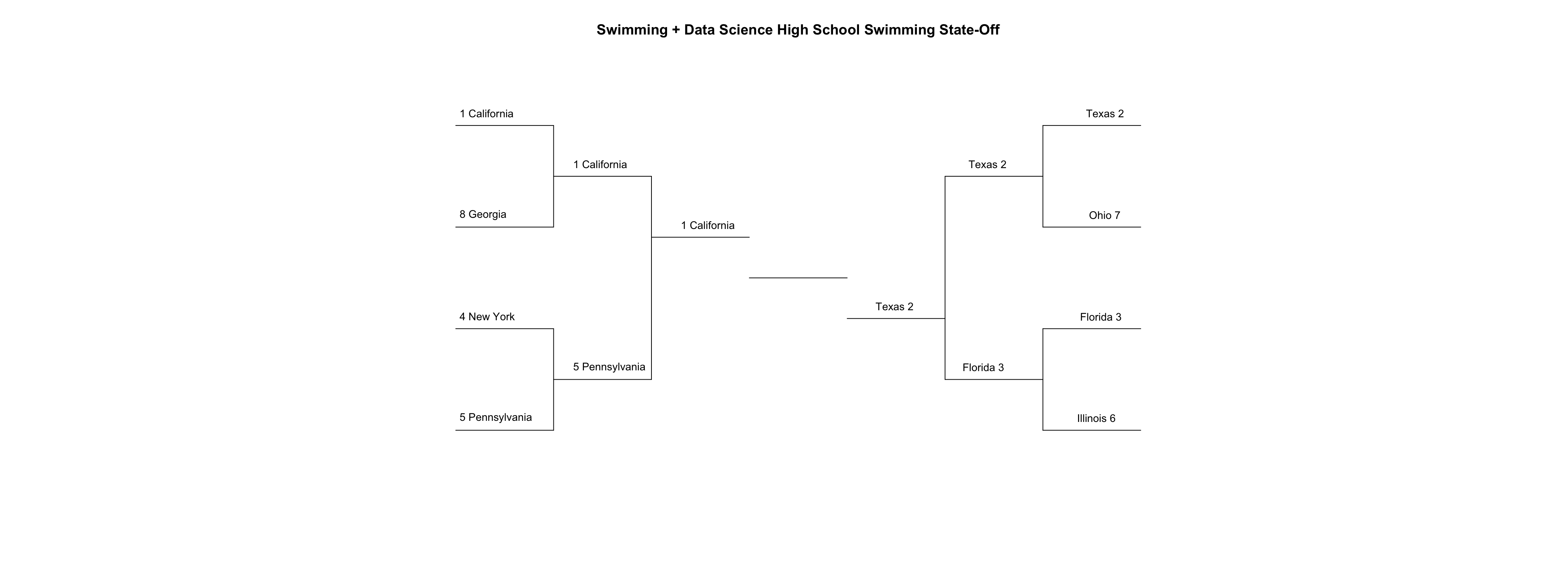
Many thanks to all of you for joining us in another round of the State-Off here at Swimming + Data Science. Next week the final State-Off Champion will be crowned. Let’s update our bracket and prepare ourselves for a 1-2 matchup between California (1) and Texas (2)!
draw_bracket(
  teams = c(
    "California",
    "Texas",
    "Florida",
    "New York",
    "Pennsylvania",
    "Illinois",
    "Ohio",
    "Georgia"
  ),
  round_two = c("California", "Texas", "Florida", "Pennsylvania"),
  round_three = c("California", "Texas"),
  title = "Swimming + Data Science High School Swimming State-Off",
  text_size = 0.9
)
Updated: 20 April, 2021
Created: 10 September, 2020