Getting Results

As I mentioned in the SwimmeR 0.4.1 post last week these posts are no longer going to focus on using SwimmeR to read in results. That’s been covered extensively in previous State-Off posts. Instead I’ve already read in the results for each state and I’m hosting them on github.

We’ll just pull results for Texas and Florida, and then stick them together with bind_rows.

Texas_Link <-
  "https://raw.githubusercontent.com/gpilgrim2670/Pilgrim_Data/master/TX_States_2020.csv"
Texas_Results <- read.csv(url(Texas_Link)) %>% 
  mutate(State = "TX",
         Grade = as.character(Grade))

Florida_Link <-
  "https://raw.githubusercontent.com/gpilgrim2670/Pilgrim_Data/master/FL_States_2020.csv"
Florida_Results <- read.csv(url(Florida_Link)) %>% 
  mutate(State = "FL")

Results <- Texas_Results %>%
  bind_rows(Florida_Results) %>%
  mutate(Gender = case_when(
    str_detect(Event, "Girls") == TRUE ~ "Girls",
    str_detect(Event, "Boys") == TRUE ~ "Boys"
  )) %>% 
  rename("Team" = School,
         "Age" = Grade)

Scoring the Meet

Here’s one of the new functions for SwimmeR 0.4.1. If you followed along with previous State-Off posts then you remember we developed the results_score function together during the first round. Now we get to use it in all of its released glory. results_score takes several arguments, results, which are the results to score, events, which are the events of interest, meet_type, which is either "timed_finals" or "prelims_finals". The last three, lanes, scoring_heats, and point_values are fairly self-explanatory, as the number of lanes, scoring heats, and the point values for each place respectively.

For the State_Off we’ve been using a "timed_finals" meet type, with 8 lanes, 2 scoring heats and point values per NFHS.

Results_Final <- results_score(
  results = Results,
  events = unique(Results$Event),
  meet_type = "timed_finals",
  lanes = 8,
  scoring_heats = 2,
  point_values = c(20, 17, 16, 15, 14, 13, 12, 11, 9, 7, 6, 5, 4, 3, 2, 1)
)

Scores <- Results_Final %>%
  group_by(State, Gender) %>%
  summarise(Score = sum(Points))

Scores %>%
  arrange(Gender, desc(Score)) %>%
  ungroup() %>%
  flextable_style()

We have our first split result of of the State-Off, with the Texas boys and Florida girls each winning. This is a combined affair though, so let’s see which state will advance…

Scores %>%
  group_by(State) %>%
  summarise(Score = sum(Score)) %>%
  arrange(desc(Score)) %>%
  ungroup() %>%
  flextable_style()

And it’s Texas, living up to it’s higher seed!

Swimmers of the Meet

Swimmer of the Meet criteria is the same as it’s been for the entire State-Off. First we’ll look for athletes who won two events, thereby scoring a the maximum possible forty points. We’ll also grab the All-American cuts to use as a tiebreaker, in case multiple athletes win two events. It’s possible this week we’ll have our first multiple Swimmer of the Meet winner - the suspense!

Cuts_Link <-
  "https://raw.githubusercontent.com/gpilgrim2670/Pilgrim_Data/master/State_Cuts.csv"
Cuts <- read.csv(url(Cuts_Link))

Cuts <- Cuts %>% # clean up Cuts
  filter(Stroke %!in% c("MR", "FR", "11 Dives")) %>% # %!in% is now included in SwimmeR
  rename(Gender = Sex) %>%
  mutate(
    Event = case_when((Distance == 200 & #match events
                         Stroke == 'Free') ~ "200 Yard Freestyle",
                      (Distance == 200 &
                         Stroke == 'IM') ~ "200 Yard IM",
                      (Distance == 50 &
                         Stroke == 'Free') ~ "50 Yard Freestyle",
                      (Distance == 100 &
                         Stroke == 'Fly') ~ "100 Yard Butterfly",
                      (Distance == 100 &
                         Stroke == 'Free') ~ "100 Yard Freestyle",
                      (Distance == 500 &
                         Stroke == 'Free') ~ "500 Yard Freestyle",
                      (Distance == 100 &
                         Stroke == 'Back') ~ "100 Yard Backstroke",
                      (Distance == 100 &
                         Stroke == 'Breast') ~ "100 Yard Breaststroke",
                      TRUE ~ paste(Distance, "Yard", Stroke, sep = " ")
    ),
    
    Event = case_when(
      Gender == "M" ~ paste("Boys", Event, sep = " "),
      Gender == "F" ~ paste("Girls", Event, sep = " ")
    )
  )

Ind_Swimming_Results <- Results_Final %>%
  filter(str_detect(Event, "Diving|Relay") == FALSE) %>% # join Ind_Swimming_Results and Cuts
  left_join(Cuts %>% filter((Gender == "M" &
                               Year == 2020) |
                              (Gender == "F" &
                                 Year == 2019)) %>%
              select(AAC_Cut, AA_Cut, Event),
            by = 'Event')

Swimmer_Of_Meet <- Ind_Swimming_Results %>%
  mutate(
    AA_Diff = (Finals_Time_sec - sec_format(AA_Cut)) / sec_format(AA_Cut),
    Name = str_to_title(Name)
  ) %>%
  group_by(Name) %>%
  filter(n() == 2) %>% # get swimmers that competed in two events
  summarise(
    Avg_Place = sum(Place) / 2,
    AA_Diff_Avg = round(mean(AA_Diff, na.rm = TRUE), 3),
    Gender = unique(Gender),
    State = unique(State)
  ) %>%
  arrange(Avg_Place, AA_Diff_Avg) %>%
  group_split(Gender) # split out a dataframe for boys (1) and girls (2)

Boys

Swimmer_Of_Meet[[1]] %>%
  slice_head(n = 5) %>%
  select(-Gender) %>%
  ungroup() %>%
  flextable_style()

Joshua Zuchowski is the boys swimmer of the meet. He’s a new face for this particular award - in Florida’s first round meet he finished third behind two guys from Illinois. Also no boy won two events.

Results_Final %>%
  filter(Name == "Zuchowski, Joshua") %>%
  select(Place, Name, Team, Finals_Time, Event) %>%
  arrange(desc(Event)) %>%
  ungroup() %>%
  flextable_style()

Girls

Swimmer_Of_Meet[[2]] %>%
  slice_head(n = 5) %>%
  select(-Gender) %>%
  ungroup() %>%
  flextable() %>%
  bold(part = "header") %>%
  bg(bg = "#D3D3D3", part = "header") %>%
  autofit()

Lillie Nordmann continues her winning ways, being named girls swimmer of the meet for the second meet in a row. While she hasn’t written in to answer my questions about swimming outdoors in cold weather she did tell SwimSwam that she’s postponing her collegiate career because of the ongoing pandemic. I don’t blame her. As these results attest, she’s a champ, and frankly this way she’ll be able to focus more on trying to make the Olympic team. Also, it’s warmer in Texas than it is in Palo Alto (or nearby San Jose). Just saying. Actually I’m not just saying - I have data on the temperatures in San Jose and Houston, from the National Weather Service. Let me show you what I’m talking about, in both Fahrenheit and Celsius (the State-Off has a surprisingly international audience).

San_Jose_Link <- "https://raw.githubusercontent.com/gpilgrim2670/Pilgrim_Data/master/San_Jose_Temps.csv"
San_Jose <- read.csv(url(San_Jose_Link)) %>% 
  mutate(City = "San Jose")
Houston_Link <- "https://raw.githubusercontent.com/gpilgrim2670/Pilgrim_Data/master/Houston_Temps.csv"
Houston <- read.csv(url(Houston_Link)) %>% 
  mutate(City = "Houston")

Temps <- bind_rows(San_Jose, Houston)

names(Temps) <- c("Month", "Mean_Max", "Mean_Min", "Mean_Avg", "City")

Temps$Month <- factor(Temps$Month, ordered = TRUE, 
                                levels = unique(Temps$Month))

Temps %>%
  ggplot() +
  geom_line(aes(
    x = Month,
    y = Mean_Avg,
    group = City,
    color = City
  )) +
  scale_y_continuous(sec.axis = sec_axis( ~ (. - 32) * (5/9), name = "Monthly Mean Average Temperature (C)")) +
  theme_bw() +
  theme(axis.text.x = element_text(angle = 45, hjust = 1)) +
  labs(x = "Month", y = "Monthly Mean Average Temperature (F)")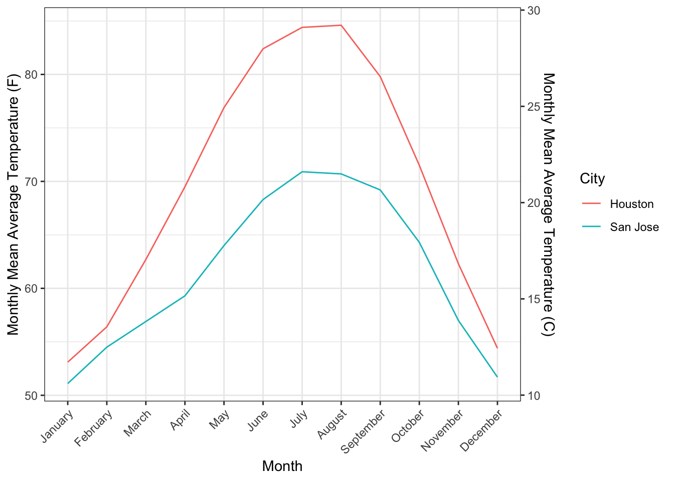

Those are the monthly average temperatures. Plotting Mean_Min is even colder, and closer to what it feels like in those early mornings. If I was going to swim outdoors I’d much rather do it in Texas versus shivering in NorCal. I am a delicate flower.

Results_Final %>%
  filter(Name == "Lillie Nordmann") %>%
  select(Place, Name, Team, Finals_Time, Event) %>%
  arrange(desc(Event)) %>%
  ungroup() %>%
  flextable_style()

The DQ Column

A new feature in SwimmeR 0.4.1 is that results now include a column called DQ. When DQ == 1 a swimmer or relay has been disqualified. Recording DQs is of course important to the overall mission of SwimmeR (making swimming results available in usable formats etc. etc.), but it’s also of personal interest to me as an official.

Results %>%
  group_by(State) %>%
  summarise(DQs = sum(DQ, na.rm = TRUE) / n()) %>%
  flextable_style()

Results %>% 
  mutate(Event = str_remove(Event, "Girls |Boys ")) %>% 
  group_by(Event) %>% 
  summarise(DQs = sum(DQ, na.rm = TRUE)) %>%
  filter(DQs > 0) %>% 
  arrange(desc(DQs)) %>% 
  head(5) %>% 
  flextable_style()

Not surprisingly most DQs are seen in relays. False starts can and do happen as teams push for every advantage. The line between a fast start and a false start is exceedingly fine. No one is trying to false start, it just happens sometimes. Breaststroke on the other hand is a disciple where intentional cheating can and sometimes does prosper. Recall Cameron van der Burgh admitting to taking extra dolphin kicks after winning gold in Rio, or Kosuke Kitajima having “no response” to Aaron Peirsol’s accusation (backed up by video) that he took an illegal dolphin kick en route to gold in Beijing. Breaststrokers also seem to struggle with the modern “brush” turn, and ring up a lot of one-hand touches. The Texas results (5A, 6A) actually say what infraction was committed, and it’s the usual mix of kicking violations and one hand touches. Florida doesn’t share reasons for DQs, but just from my own experience - kicking and one hand touches. Must be in the water. Or not, because butterflyers don’t seem to suffer from the same issues. Could be the the butterfly recovery is more difficult to stop short, or to do in an unbalanced fashion such that only one hand makes contact with the wall? I don’t know, it’s an genuine mystery, but it is nice that my personal observations from officiating are borne out in the data.

Plotting Times With SwimmeR

We might be interested in seeing a distribution of times for a particular event. There’s a problem though. Swimming times are traditionally reported as minutes:seconds.hundredths. In R that means they’re stored as character strings, which can be confirmed by calling str(Results$Finals_Time). We’d like to be able to look at times from fastest to slowest though - that is we’d like them to have an order. One option would be to convert the character strings in Results$Finals_Time to an ordered factor, but that would be awful. We’d likely need to manually define the ordering - no fun at all. SwimmeR instead offers a pair of functions to make this easier. The function sec_format will take a time written as minutes:seconds.hundredths, like the ones in Results$Finals_Time and covert it to a numeric value - the total duration in seconds. Ordering numerics is easy, R handles it automatically. While that’s very nice, we as swimming aficionados would still like to look at times in the standard swimming format. This is where mmss_format comes in - it simply coverts times back to the standard minutes:seconds.hundredths for our viewing pleasure. Below is an example of converting times to numeric with sec_format for plotting, and then converting the axis labels to swimming format with mmss_format for viewing.

Results %>%
  filter(Gender == 'Girls',
         str_detect(Event, "Relay") == FALSE) %>%
  left_join(Cuts %>% filter(Year == 2019, Gender == "F"), by = c("Event")) %>% # add in All-American cuts
  filter(Event == "Girls 200 Yard Freestyle") %>% # pick event
  mutate(Finals_Time = sec_format(Finals_Time)) %>% # change time format to seconds
  ggplot() +
  geom_histogram(aes(x = Finals_Time, fill = State), binwidth = 0.5) +
  geom_vline(aes(xintercept = sec_format(AA_Cut))) + # line for All-American cut
  geom_vline(aes(xintercept = sec_format(AAC_Cut))) + # line for All-American consideration cut
  scale_y_continuous(breaks = seq(0, 10, 2)) +
  scale_x_continuous(
    breaks = seq(100, 150, 5),
    labels = scales::trans_format("identity", mmss_format) # labels in swimming format
  ) +
  geom_label(
    label = "All-American",
    x = 107,
    y = 7,
    color = "black"
  ) +
  geom_label(
    label = "All-American Cons.",
    x = 110.5,
    y = 10,
    color = "black"
  ) +
  theme_bw() +
  labs(y = "No. of Swimmers",
       x = "Finals Time")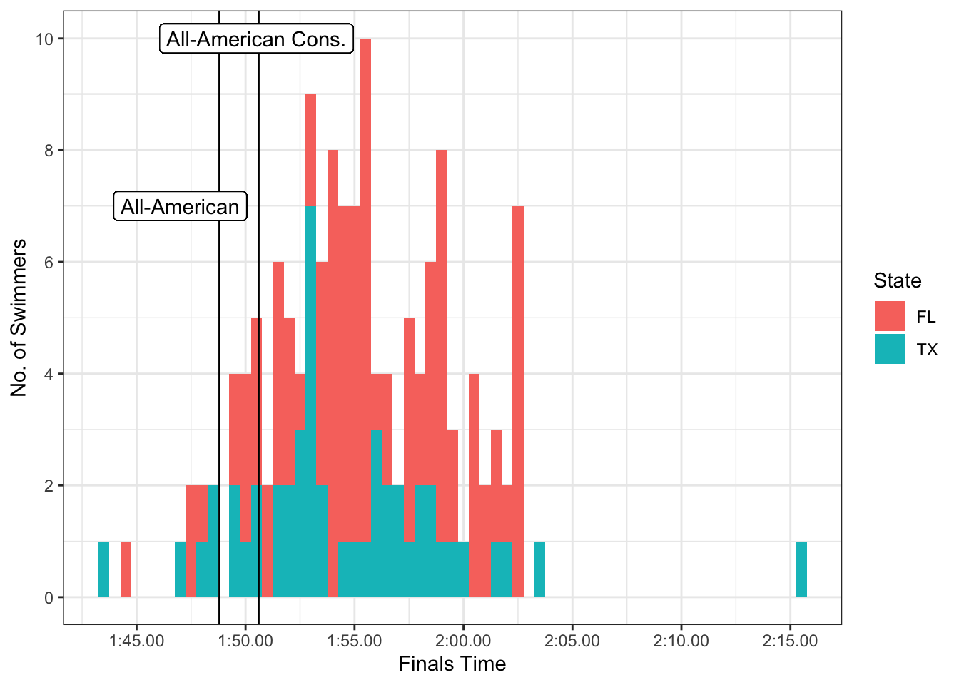

Here we see classic “bell” curves for each state, with a few very fast or very slow (comparatively speaking) swimmers, and a bunch of athletes clumped right in the middle.

In Closing

Texas wins the overall, despite a winning effort from the Florida girls. Next week at Swimming + Data Science we’ll have number one seed California (1) vs. number five Pennsylvania (5). We’ll also dig further into new SwimmeR 0.4.1 functionality. Hope to see you then!