The 2021 USMS ePostal Championship Results, Working Up Data for a Shiny App
Final results for the 2021 USMS ePostal National Championships have been posted. We’ll take a look at them using some basic summary stats and charts, then work up the data from inclusion in Shiny application built to present it interactively.
If you’d like to just skip to playing with the app and not bother about working up the data the app is available here.
This will be a tutorial style post, where I’ll prioritize making the code clear and readable, while perhaps sacrificing efficiency. No building functions and them mapping them like I sometimes do.
With that in mind let’s grab some packages. We’ll use readr to actually read in the data set. Then dplyr and stringr to work it up and finally ggplot2 and flextable to present it at various points throughout the article.
library(readr)
library(dplyr)
library(stringr)
library(ggplot2)
library(flextable)


flextable_style <- function(x) {
  x %>%
    flextable() %>%
    bold(part = "header") %>% # bolds header
    bg(bg = "#D3D3D3", part = "header") %>%  # puts gray background behind the header row
    autofit()
}
I’ve already collected the data from USMS, wrestled it into a .csv file and hosted that on Github (you’re all very welcome). We can grab it directly with read_csv.
Postal <- read_csv("https://raw.githubusercontent.com/gpilgrim2670/MastersPostal/master/Postal_Raw.csv")Last year I did a big analysis of the 2020 ePostal results and another on the ePostal over the past two+ decades. Rather than just repurposing all that code (which you’re welcome to do if you’d like) we’ll just take a quick look at the 2021 results before working up all the data, from all the years for the Shiny app.
How Many People Participated This Year?
Postal %>%
  filter(Year == "2021") %>%
  group_by(Gender) %>%
  summarise(Count = n()) %>%
  flextable_style()
Gender | Count |
M | 317 |
W | 372 |
How Does That Compare to Previous Years?
Postal %>%
  group_by(Year, Gender) %>%
  summarise(Count = n()) %>%
  ggplot() +
  geom_line(aes(x = Year, y = Count, color = Gender)) +
  theme_bw() +
  labs(title = "USMS ePostal Participation by Year")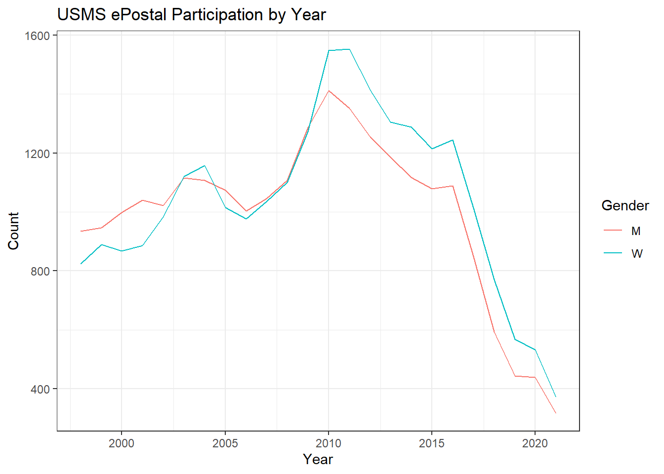
It’s fewer people. Probably COVID, and the general trends discussed here. Moving on.
Shiny App
Cleaning Data for a Shiny App
The data we’ve already downloaded and named Postal contains the as-reported results from all ePostals from 1998 through 2021. Let’s take a look.
names(Postal)## [1] "Place" "Name" "Age" "USMS_ID"
## [5] "Distance" "Club" "Gender" "Year"
## [9] "National_Record"Pretty self explanatory column names, and quite a bit of information. There’s more though that we can tease out.
I’d like to add to Postal in the following ways:
- Age groups. The ePostal is scored by age group, 18-24 and then by 5 year windows thereafter (25-29 etc.)
- Athlete’s relative place within their age and gender category by year
- An athlete’s average 50 split, based on distance traveled and assuming a 25 yard pool
- Cleaning up USMS identification to identify athletes across years
- Club sizes. USMS defines club sizes and scores based on those sizes, both by gender and total size by year
- Summary stats for clubs by year
- Total distance swam
- Club rankings by gender
- Average distance traveled and 50 split by gender
- Average age by gender
Since this is headed for a Shiny app, where it will be displayed the goal will be to make information readable, which will involve some sacrifices. For example an athlete’s relative place will be a string in the form of “Athlete place of Total place” (i.e. “1 of 54”) rather than just a naked numeric.
Age Groups
Since we already have an Age column making an age group column is a simple matter of using dplyr::case_when to match the appropriate age range to the Age. We’ll do this using dplyr::between. between takes three arguments - a value x, a left and a right. If x >= left & x <= right then between returns TRUE. Otherwise between returns FASLE. The resulting code is perhaps long, and there are more compact ways to do this, but it’s also very readable, approximating written English. Readability is useful in the context of a blog entry and I’ll continue to prioritize it throughout.
Postal <- Postal %>%
  mutate(
    Age_Group = case_when(
      between(Age, 0, 24) ~ "18-24",
      between(Age, 25, 29) ~ "25-29",
      between(Age, 30, 34) ~ "30-34",
      between(Age, 35, 39) ~ "35-39",
      between(Age, 40, 44) ~ "40-44",
      between(Age, 45, 49) ~ "45-49",
      between(Age, 50, 54) ~ "50-54",
      between(Age, 55, 59) ~ "55-59",
      between(Age, 60, 64) ~ "60-64",
      between(Age, 65, 69) ~ "65-69",
      between(Age, 70, 74) ~ "70-74",
      between(Age, 75, 79) ~ "75-79",
      between(Age, 80, 84) ~ "80-84",
      between(Age, 85, 89) ~ "85-89",
      between(Age, 90, 94) ~ "90-94",
      between(Age, 95, 99)~ "95-99",
      between(Age, 100, 104) ~ "100-104",
      TRUE ~ "NA" # if for some reason Age doesn't match any of the above this will catch it and write the string 'NA'
    )
  ) %>%
  mutate(Age_Group = factor(Age_Group, levels = c("18-24", "25-29", "30-34", "35-39", "40-44", "45-49", "50-54", "55-59", "60-64", "65-69", "70-74", "75-79", "80-84", "85-89", "90-94", "95-99")))

# demonstration table
Postal %>%
  select(Place, Name, Distance, Year, Age, Age_Group, Gender) %>%
  head(5) %>%
  flextable_style()
Place | Name | Distance | Year | Age | Age_Group | Gender |
1 | Robert Wagner | 5450 | 2021 | 19 | 18-24 | M |
2 | Elliott Roman | 5215 | 2021 | 24 | 18-24 | M |
3 | William Kemp | 4700 | 2021 | 22 | 18-24 | M |
4 | Dylan Ogle | 4250 | 2021 | 23 | 18-24 | M |
5 | Gregory Willett | 4035 | 2021 | 24 | 18-24 | M |
Athlete Relative Place
As discussed above the athlete place column will contain a string giving an individual athlete’s place within their age and gender category for a given year. The point is to provide a means of comparing two athletes in the Shiny app. If Athlete A and Athlete B both finished 6th, but Athlete A did so in a category with 50 entrants vs. only 10 in Athlete B’s category then that’s worth knowing when comparing them.
Here we’ll just paste an athlete’s Place, the string " of " and the maximumn place from that age group together.
Postal <- Postal %>%
  group_by(Gender, Age_Group, Year) %>% # places are caluclated by gender, age group and year
  mutate(Relative_Place = paste(Place, max(Place, na.rm = TRUE), sep = " of ")) # use paste to build string

# demonstration table
Postal %>%
  select(Place, Name, Distance, Year, Age_Group, Gender, Relative_Place) %>%
  head(5) %>%
  flextable_style()
Place | Name | Distance | Year | Age_Group | Gender | Relative_Place |
1 | Robert Wagner | 5450 | 2021 | 18-24 | M | 1 of 5 |
2 | Elliott Roman | 5215 | 2021 | 18-24 | M | 2 of 5 |
3 | William Kemp | 4700 | 2021 | 18-24 | M | 3 of 5 |
4 | Dylan Ogle | 4250 | 2021 | 18-24 | M | 4 of 5 |
5 | Gregory Willett | 4035 | 2021 | 18-24 | M | 5 of 5 |
Average 50 Split
I’m accustomed to looking at 50 splits in swimming, and I think it’s an interesting metric by which to evaluate ePostal results as well. An athlete’s split can be calculated by converting the time (1 hour), then multiplying that number of seconds by 50 and then multiplying again by reciprocal distance to get a number in units of seconds per 50 yards. We can then round and format the result to make it pleasant to look at.
Postal <- Postal %>%
  mutate(Avg_Split_50 = (1 / Distance) * 60 * 60 * 50) %>% # compute split
  mutate(Avg_Split_50 = format(round(Avg_Split_50, 2), nsmall = 2)) # want two decimal places, even if the last one is a zero

# demonstration table
Postal %>%
  select(Place, Name, Distance, Year, Age_Group, Gender, Avg_Split_50) %>%
  head(5) %>%
  flextable_style()
Place | Name | Distance | Year | Age_Group | Gender | Avg_Split_50 |
1 | Robert Wagner | 5450 | 2021 | 18-24 | M | 33.03 |
2 | Elliott Roman | 5215 | 2021 | 18-24 | M | 34.52 |
3 | William Kemp | 4700 | 2021 | 18-24 | M | 38.30 |
4 | Dylan Ogle | 4250 | 2021 | 18-24 | M | 42.35 |
5 | Gregory Willett | 4035 | 2021 | 18-24 | M | 44.61 |
USMS_ID
The value in USMS_ID has two parts. The first four characters, before the "-" vary year to year. The last five characters, after the "-" are an athlete’s permanent identification string, used to identify athletes without relaying on names. We discuss this records matching problem a lot around here, because athlete names aren’t a stable means of identification. Sometimes people get married and change their names. Sometimes people use nicknames. Things happen and the permanant portion of the USMS_ID is a good way of handling things. Sadly ePostal results only include USMS_ID after 2010, so we need to come up with something for pre-2011 results.
Here’s the plan. We’ll break off the permanent portion of USMS_ID into a new column called Perm_ID based on the location of "-" using str_split_fixed. Rows without a USMS_ID will have an empty character string "" in Perm_ID, which we’ll convert to NA with na_if. Then we’ll group athletes by name. If any entry for that athlete, using that name, is from post-2010 they’ll have a Perm_ID which we’ll be able to copy to all rows involving that name using the tidyr::fill function. It’s of course possible to have two athletes with the same name. We could be stricter here and group_by name and club for example, but athletes do change clubs. There are other things we could try as well, like matching on age progression, but for right now we’re just going to accept that there might be some false matches.
Postal <- Postal %>%
  mutate(Perm_ID = str_split_fixed(USMS_ID, "-", n = 2)[, 2], # only want the second part of the split
         Perm_ID = na_if(Perm_ID, "")) %>%  # turn empty strings "" into NAs
  group_by(Name) %>%
  tidyr::fill(Perm_ID, .direction = "updown") # all instances of name will get non-NA value of Perm_ID - assumes there's only one unique Perm_ID for each name
Some athletes still don’t have a Perm_ID though, because they don’t have a USMS_ID listed.
# demonstration table
Postal %>%
  filter(Year == 1998) %>%
  select(Place, Name, Year, USMS_ID, Perm_ID) %>%
  head(5) %>%
  flextable_style()
Place | Name | Year | USMS_ID | Perm_ID |
1 | Becky Crowe | 1998 | ||
2 | Johanna Hardin | 1998 | ||
3 | Sarah Anderson | 1998 | ||
4 | Sarah Baker | 1998 | 09RB9 | |
5 | Jane Kelsey | 1998 |
We’re going to make them fake Perm_IDs. Each fake Perm_ID will be a six character string of upper case letters. We’ll use this slightly different format (compared to the five character alphanumeric real Perm_IDs) so that it’s possible to differentiate the fake from the real.
Each unique name without a real Perm_ID needs a fake Perm_ID. Let’s first collect those unique names.
Unique_Names <- Postal %>%
  ungroup() %>%
  select(Name, Perm_ID) %>% # don't need all the columns, only these two
  filter(is.na(Perm_ID) == TRUE) %>% # want only rows where there isn't a Perm_ID
  unique() # don't need duplicates

Unique_Names %>%
  head(5) %>%
  flextable_style()
Name | Perm_ID |
Glen Christiansen | |
Lou Hill | |
Sue Lyon | |
Masao Miyasaka | |
Karina Horton |
Now we need a list of random strings, one for each name. Since we’re generating something random we’ll use set.seed to make it reproducible. Then we’ll use the stringi::stri_rand_strings function to generate a list of random strings with length 6. The length of the list will be the number of rows in unique_names.
set.seed(1) # to make random strings reproducible

Unique_Names <- Unique_Names %>%
  mutate(Perm_ID = stringi::stri_rand_strings( # make random strings
    n = nrow(Unique_Names), # number of random strings to make
    length = 6, # number of characters in each string
    pattern = "[A-Z]" # what to make the string out of, in this case all capital letters
  ))

# demonstration table
Unique_Names %>%
  head(5) %>%
  flextable_style()
Name | Perm_ID |
Glen Christiansen | GJOXFX |
Lou Hill | YRQBFE |
Sue Lyon | RJUMSZ |
Masao Miyasaka | JUYFQD |
Karina Horton | GKAJWI |
Now we’ll join Postal and Unique_Names back up by Name and use coalesce to get non-NA values of Perm_ID for each row. Each Name, which hopefully means each athlete, now has a unique Perm_ID.
Postal <- Postal %>%
  left_join(Unique_Names, by = "Name") %>% # attach newly made strings back to original data frame based on name
  mutate(Perm_ID = coalesce(Perm_ID.x, Perm_ID.y)) %>% # use first non-na value between original data frame (x) and new data frame (y)
  select(-Perm_ID.x, -Perm_ID.y) # don't need these columns any more

# demonstration table
Postal %>%
  filter(Year == 1998) %>%
  select(Place, Name, Year, USMS_ID, Perm_ID) %>%
  head(5) %>%
  flextable_style()
Place | Name | Year | USMS_ID | Perm_ID |
1 | Becky Crowe | 1998 | XZPOKS | |
2 | Johanna Hardin | 1998 | EOFXZG | |
3 | Sarah Anderson | 1998 | YSAWZT | |
4 | Sarah Baker | 1998 | 09RB9 | |
5 | Jane Kelsey | 1998 | DHNSNX |
Club Sizes
USMS defines categories of club size for the ePostal as small, medium, large and extra large based on the number of athletes representing that club. Here we’ll count the number of athletes for each club with n and categorize appropriately with case_when. It’s also interesting to look at participation by gender, so we’ll count the male and female athletes for each club using sum. We’ll get new columns of the form Club_Count (number of athletes in a club) and Club_Size (a factor with levels S, M, L, XL).
# total club size
Postal <- Postal %>%
    group_by(Club, Year) %>% # working with clubs now, by year
    mutate(Club_Count = n()) %>% # number of athletes in each club for a given year
    mutate(Club_Size_Combined = case_when( # code in club sizes based on number of athletes
      Club_Count < 26 ~ "S",
      Club_Count < 50 ~ "M",
      Club_Count <= 100 ~ "L",
      TRUE ~ "XL"
    )) %>%
  mutate(Club_Size_Combined = factor(Club_Size_Combined, levels = c("S", "M", "L", "XL")))

# male club size
Postal <- Postal %>%
    group_by(Club, Year) %>%
    mutate(Club_Count_Male = sum(Gender == "M", na.rm = TRUE)) %>% # only want to count men this time
    mutate(Club_Size_Male = case_when(
      Club_Count_Male < 26 ~ "S",
      Club_Count_Male < 50 ~ "M",
      Club_Count_Male <= 100 ~ "L",
      TRUE ~ "XL"
    )) %>%
    mutate(Club_Size_Male = factor(Club_Size_Male, levels = c("S", "M", "L", "XL")))

# female club size
Postal <- Postal %>%
    group_by(Club, Year) %>%
    mutate(Club_Count_Female = sum(Gender == "W", na.rm = TRUE)) %>% # only want to count women this time
    mutate(Club_Size_Female = case_when(
      Club_Count_Female < 26 ~ "S",
      Club_Count_Female < 50 ~ "M",
      Club_Count_Female <= 100 ~ "L",
      TRUE ~ "XL"
    )) %>%
    mutate(Club_Size_Female = factor(Club_Size_Female, levels = c("S", "M", "L", "XL")))

# demonstration table
Postal %>%
  select(Club, Year, Club_Count, Club_Size_Combined, Club_Size_Male) %>%
  head(5) %>%
  flextable_style()
Club | Year | Club_Count | Club_Size_Combined | Club_Size_Male |
BSMT | 2021 | 46 | M | S |
SKY | 2021 | 15 | S | S |
SKY | 2021 | 15 | S | S |
GS | 2021 | 3 | S | S |
SKY | 2021 | 15 | S | S |
Club Summary Stats
In addition to making comparisons between athletes we can also make comparisons between clubs.
Club Total and Average Distance
Clubs are scored based on the total distance swam by their memberships. Here we can group_by club can year, then add up the total distance each club swam with sum.
# total club stats
Postal <- Postal %>%
  mutate(Distance = na_if(Distance, 0)) %>% # shouldn't be any distance NA values, but convert to zero if there are
  group_by(Club, Year) %>%
  mutate(Total_Distance_Combined = sum(Distance, na.rm = TRUE)) %>% # add up distance for each club/year
  mutate(Avg_Distance_Combined = Total_Distance_Combined / Club_Count) %>% # calculate avg distance per athlete
  mutate(Avg_Distance_Combined = round(Avg_Distance_Combined, 0))# don't want decimal places


# male stats
Postal <- Postal %>%
  group_by(Club, Year) %>%
  mutate(Total_Distance_Male = sum(Distance[Gender == "M"], na.rm = TRUE)) %>%
  mutate(Avg_Distance_Male = Total_Distance_Male / Club_Count_Male) %>%
  mutate(Avg_Distance_Male = round(Avg_Distance_Male, 0))

# female stats
Postal <- Postal %>%
  group_by(Club, Year) %>%
  mutate(Total_Distance_Female = sum(Distance[Gender == "W"], na.rm = TRUE)) %>%
  mutate(Avg_Distance_Female = Total_Distance_Female / Club_Count_Female) %>%
  mutate(Avg_Distance_Female = round(Avg_Distance_Female, 0))

# demonstration table
Postal %>%
  filter(Gender == "W") %>%
  select(Club, Year, Total_Distance_Female, Avg_Distance_Female) %>%
  head(5) %>%
  flextable_style()
Club | Year | Total_Distance_Female | Avg_Distance_Female |
IM | 2021 | 45420 | 3785 |
GS | 2021 | 5850 | 2925 |
UC08 | 2021 | 3400 | 3400 |
CRUZ | 2021 | 18475 | 4619 |
1776 | 2021 | 38340 | 4260 |
Club Rank
Clubs can be ranked within their size/gender categories by total distance swam in much the same way we ranked swimmers within their age/gender categories. Since their are only three categories (combined, male, female) I’m not going to bother about including category size like with did with individual athletes although it’s certainly possible to do so. Here we’ll just group_by the appropriate Club_size column and the year and then use dense_rank to get the ranking for each club. dense_rank is one of the the six dplyr ranking functions. It ranks values in a vector giving tied values a minimum rank and does not skip places as a result of ties. Here’s a demonstration, because some of you might not be familiar with dense_rank.
Assume four clubs A-D, each of which swam some total distance.
distances <- c(10000, 15000, 15000, 20000)
names(distances) <- c("A", "B", "C", "D")
distances
## A B C D
## 10000 15000 15000 20000What we’d like to say is that club D is first, clubs B and C are tied for second and club A is third. Club B and C both getting second (rather than say, 2.5th, or randomly giving one 2nd and the other 3rd) is what I mean by “giving tied values a minimum rank”. Club A getting third, rather than forth (as the forth club on the list) is what I mean by “not skip[ping] places as a result of ties”. We also need to use desc because we want the clubs with the largest distance values to get the lowest valued places - club D should be first.
dense_rank(desc(distances))## [1] 3 2 2 1Now to use dense_rank with our real data.
# total club stats
Postal <- Postal %>%
  group_by(Club_Size_Combined, Year) %>%
  mutate(Combined_Rank = dense_rank(desc(Total_Distance_Combined))) # calculate ranking

# male stats
Postal <- Postal %>%
  group_by(Club_Size_Male, Year) %>%
  mutate(Male_Rank = dense_rank(desc(Total_Distance_Male)))


# female stats
Postal <- Postal %>%
  group_by(Club_Size_Female, Year) %>%
  mutate(Female_Rank = dense_rank(desc(Total_Distance_Female)))

# demonstration table
Postal %>%
  filter(Gender == "W") %>%
  select(Club,
         Year,
         Club_Size_Female,
         Total_Distance_Female,
         Female_Rank) %>%
  head(5) %>%
  flextable_style()
Club | Year | Club_Size_Female | Total_Distance_Female | Female_Rank |
IM | 2021 | S | 45420 | 5 |
GS | 2021 | S | 5850 | 44 |
UC08 | 2021 | S | 3400 | 67 |
CRUZ | 2021 | S | 18475 | 14 |
1776 | 2021 | S | 38340 | 8 |
Average Club Splits
Average club splits are similar to athlete splits, just for an entire club. There are lots of ways to calculate such a value. We could group_by club and average the Avg_Split_50 that we already calculated. Or we could recalculate based on Avg_Club_Distance. Let’s do that.
# total club splits
Postal <- Postal %>%
  ungroup() %>%
  group_by(Club, Year) %>%
  mutate(Avg_Split_50_Club_Combined = (1 / Avg_Distance_Combined) * 60 * # compute 50 splits by club, year
           60 * 50) %>%
  mutate(Avg_Split_50_Club_Combined = format(round(Avg_Split_50_Club_Combined, 2), nsmall = 2))

# male club splits
Postal <- Postal %>%
  ungroup() %>%
  group_by(Club, Year) %>%
  mutate(Avg_Split_50_Club_Male = (1 / Avg_Distance_Male) * 60 * 60 *
           50) %>%
  mutate(Avg_Split_50_Club_Male =
           format(round(Avg_Split_50_Club_Male, 2), nsmall = 2))

# female club splits
Postal <- Postal %>%
  ungroup() %>%
  group_by(Club, Year) %>%
  mutate(Avg_Split_50_Club_Female = (1 / Avg_Distance_Female) * 60 * 60 *
           50) %>%
  mutate(Avg_Split_50_Club_Female =
           format(round(Avg_Split_50_Club_Female, 2), nsmall = 2))

# demonstration table
Postal %>%
  filter(Gender == "W") %>%
  arrange(desc(Avg_Distance_Female)) %>%
  select(Club,
         Year,
         Club_Size_Female,
         Avg_Split_50_Club_Female,
         Female_Rank) %>%
  head(5) %>%
  flextable_style()
Club | Year | Club_Size_Female | Avg_Split_50_Club_Female | Female_Rank |
CFMS | 2015 | S | 33.12 | 88 |
UHM | 2000 | S | 33.77 | 55 |
LVM | 2009 | S | 34.42 | 75 |
TERA | 1999 | S | 34.42 | 51 |
ALEX | 2014 | S | 34.45 | 105 |
Average Club Age
Here we’ll go the other way, and compute average club ages by grouping_by Club and Year and then taking the mean of Age for all athletes in each group.
# total club age
Postal <- Postal %>%
  group_by(Club, Year) %>%
  mutate(Avg_Age_Club = mean(Age, na.rm = TRUE)) %>% # average age of club athletes in a given year
  mutate(Avg_Age_Club = round(Avg_Age_Club, 2)) # round off to 2 decimal places


# male club age
Postal <- Postal %>%
  group_by(Club, Year) %>%
  mutate(Avg_Age_Club_Male = mean(Age[Gender == "M"], na.rm = TRUE)) %>%
  mutate(Avg_Age_Club_Male = round(Avg_Age_Club_Male, 2))

# female club age
Postal <- Postal %>%
  group_by(Club, Year) %>%
  mutate(Avg_Age_Club_Female = mean(Age[Gender == "W"], na.rm = TRUE)) %>%
  mutate(Avg_Age_Club_Female = round(Avg_Age_Club_Female, 2))

# demonstration table
Postal %>%
  arrange(Avg_Age_Club) %>%
  select(Club,
         Year,
         Club_Size_Combined,
         Avg_Age_Club,
         Combined_Rank) %>%
  head(5) %>%
  flextable_style()
Club | Year | Club_Size_Combined | Avg_Age_Club | Combined_Rank |
BAY | 2013 | S | 19 | 129 |
SBAS | 2006 | S | 19 | 78 |
UCSB | 2006 | S | 20 | 79 |
CHR | 2005 | S | 20 | 88 |
GSC | 2001 | S | 20 | 95 |
A Shiny App
We’re not going to build a Shiny app here, but I’ll show you one I’ve already built that runs off this data. You can explore it here and view the source code here. Please note I only have so much bandwidth available for the Shiny app. If it doesn’t open for you try again later. Below are some screen shots of the app in action.
It will let you view results from individual athletes and/or whole clubs over the years:
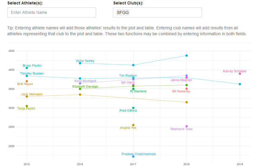
Screenshot of Timeseries Plot for SFGG Athletes
Or box plots by gender for a given year, similar to this post:
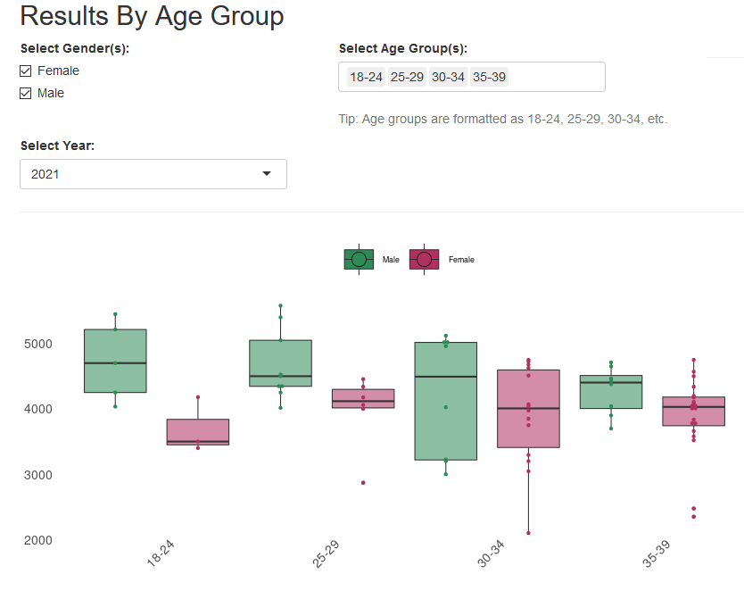
Screenshot of Box Plots for Age Groups by Gender in 2021
Or a table of club results for a given year:
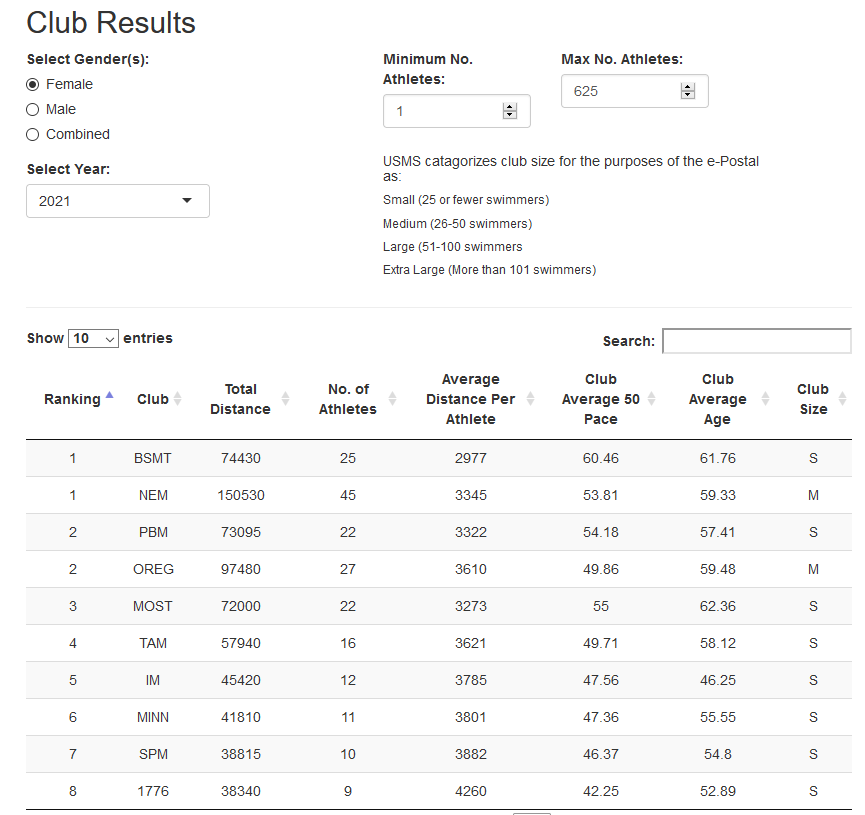
Screenshot of Club Results Table 2021
All the data is downloadable as .csv files directly from the app.
Conclusions
Thank you for joining us here at Swimming + Data Science for what’s hopefully been an informative look at working up data and the USMS ePostal. Come back and join us next time when we’ll be doing - something else. I’m not quite sure yet.
Updated: 27 April, 2021
Created: 27 April, 2021