High School Swimming State-Off Tournament Championship California (1) vs. Texas (2)
This is it folks, the big one, the finals of the State-Off Tournament, where we’ll see California (1) take on Texas (2) for high school swimming superiority. We’ll also use a t-test to determine whether or not swimmers actually swim faster in finals sessions, when the pressure is on. Oh and it’s so on!
library(SwimmeR)
library(dplyr)
library(stringr)
library(flextable)
library(ggplot2)
Please note the following analysis was updated November 22nd 2020 to reflect changes beginning with SwimmeR v0.6.0 released via CRAN on November 22nd 2020. Please make sure your version of SwimmeR is up-to-date.
My flextable styling function is still working great since I made it two weeks ago. In the finals you’ve just gotta stick with what works.
flextable_style <- function(x) {
  x %>%
    flextable() %>%
    bold(part = "header") %>% # bold header
    bg(bg = "#D3D3D3", part = "header") %>% # puts gray background behind the header row
    autofit()
}
Getting Results
The suspense is killing me here! Let’s get this thing underway by grabbing results from github.
California_Link <-
  "https://raw.githubusercontent.com/gpilgrim2670/Pilgrim_Data/master/CA_States_2019.csv"
California_Results <- read.csv(url(California_Link)) %>%
  mutate(State = "CA")
Texas_Link <-
"https://raw.githubusercontent.com/gpilgrim2670/Pilgrim_Data/master/TX_States_2020.csv"
Texas_Results <- read.csv(url(Texas_Link)) %>%
mutate(State = "TX",
Grade = as.character(Grade))Results <- California_Results %>%
bind_rows(Texas_Results) %>%
mutate(Gender = case_when(
str_detect(Event, "Girls") == TRUE ~ "Girls",
str_detect(Event, "Boys") == TRUE ~ "Boys"
)) %>%
rename("Age" = Grade,
"Team" = School)
Scoring the Meet
Results_Final <- results_score(
  results = Results,
  events = unique(Results$Event),
  meet_type = "timed_finals",
  lanes = 8,
  scoring_heats = 2,
  point_values = c(20, 17, 16, 15, 14, 13, 12, 11, 9, 7, 6, 5, 4, 3, 2, 1)
)

Scores <- Results_Final %>%
  group_by(State, Gender) %>%
  summarise(Score = sum(Points))

Scores %>%
  arrange(Gender, desc(Score)) %>%
  ungroup() %>%
flextable_style()State | Gender | Score |
CA | Boys | 1,516.5 |
TX | Boys | 808.5 |
CA | Girls | 1,454.0 |
TX | Girls | 871.0 |
Scores %>%
  group_by(State) %>%
  summarise(Score = sum(Score)) %>%
  arrange(desc(Score)) %>%
  ungroup() %>%
flextable_style()State | Score |
CA | 2,970.5 |
TX | 1,679.5 |
In an outcome that many of you probably predicted ahead of time, California (1) lives up to their number one ranking and secures State-Off Tournament crown over Texas (2). Just because it was expected though doesn’t meet it’s not impressive. This meet was super fast. Let’s look at some individual performances and name our Swimmers of the Meet.
Swimmers of the Meet
Two swimmers come into this meet on Swimmer of the Meet streaks. Lillie Nordmann has won two in row for the Texas girls, and Zoie Hartman has won two in a row for the California girls. Swimmer of the Meet criteria is still the same as it’s been for the entire State-Off. We’ll look for athletes who have won two events, thereby scoring a the maximum possible forty points. In the event of a tie, where multiple athletes win two events, we’ll use All-American standards as a tiebreaker.
Cuts_Link <-
  "https://raw.githubusercontent.com/gpilgrim2670/Pilgrim_Data/master/State_Cuts.csv"
Cuts <- read.csv(url(Cuts_Link))

Cuts <- Cuts %>% # clean up Cuts
  filter(Stroke %!in% c("MR", "FR", "11 Dives")) %>% # %!in% is now included in SwimmeR
  rename(Gender = Sex) %>%
  mutate(
    Event = case_when((Distance == 200 & #match events
                         Stroke == 'Free') ~ "200 Yard Freestyle",
                      (Distance == 200 &
                         Stroke == 'IM') ~ "200 Yard IM",
                      (Distance == 50 &
                         Stroke == 'Free') ~ "50 Yard Freestyle",
                      (Distance == 100 &
                         Stroke == 'Fly') ~ "100 Yard Butterfly",
                      (Distance == 100 &
                         Stroke == 'Free') ~ "100 Yard Freestyle",
                      (Distance == 500 &
                         Stroke == 'Free') ~ "500 Yard Freestyle",
                      (Distance == 100 &
                         Stroke == 'Back') ~ "100 Yard Backstroke",
                      (Distance == 100 &
                         Stroke == 'Breast') ~ "100 Yard Breaststroke",
                      TRUE ~ paste(Distance, "Yard", Stroke, sep = " ")
    ),

    Event = case_when(
      Gender == "M" ~ paste("Boys", Event, sep = " "),
      Gender == "F" ~ paste("Girls", Event, sep = " ")
    )
  )

Ind_Swimming_Results <- Results_Final %>%
  filter(str_detect(Event, "Diving|Relay") == FALSE) %>% # join Ind_Swimming_Results and Cuts
  left_join(Cuts %>% filter((Gender == "M" &
                               Year == 2020) |
                              (Gender == "F" &
                                 Year == 2019)) %>%
              select(AAC_Cut, AA_Cut, Event),
            by = 'Event')

Swimmer_Of_Meet <- Ind_Swimming_Results %>%
  mutate(
    AA_Diff = (Finals_Time_sec - sec_format(AA_Cut)) / sec_format(AA_Cut),
    Name = str_to_title(Name)
  ) %>%
  group_by(Name) %>%
  filter(n() == 2) %>% # get swimmers that competed in two events
  summarise(
    Avg_Place = sum(Place) / 2,
    AA_Diff_Avg = round(mean(AA_Diff, na.rm = TRUE), 3),
    Gender = unique(Gender),
    State = unique(State)
  ) %>%
  arrange(Avg_Place, AA_Diff_Avg) %>%
  group_split(Gender) # split out a dataframe for boys (1) and girls (2)
Boys
Swimmer_Of_Meet[[1]] %>%
  slice_head(n = 5) %>%
  select(-Gender) %>%
  ungroup() %>%
flextable_style()Name | Avg_Place | AA_Diff_Avg | State |
Hu, Ethan | 1.0 | -0.052 | CA |
Dillard, Ben | 1.5 | -0.044 | CA |
Saunders, Max | 1.5 | -0.030 | CA |
Mefford, Colby | 1.5 | -0.027 | CA |
Lee, Connor | 2.0 | -0.029 | CA |
Ethan Hu leads a California sweep en route to winning his second Swimmer of the Meet title, following the one he earned against Georgia (8) in the first round. Ethan of course now swims for Stanford, and those of you who have been following along know that Stanford is something of trigger for me. The great school and swim program aside, I’m genuinely confused as to why anyone wants to swim outdoors in the sneakily cold Bay Area. I’ve mentioned before that I used to live, and swim, in the Bay. I hated the cold and complained about it so much that a non-swimming, long-suffering, friend was inspired to remix this Peanuts cartoon about it.

Anyways, here’s Ethan’s results:
Results_Final %>%
  filter(Name == "Hu, Ethan") %>%
  select(Place, Name, Finals_Time, Event) %>%
  arrange(desc(Event)) %>%
  ungroup() %>%
flextable_style()Place | Name | Finals_Time | Event |
1 | Hu, Ethan | 1:45.44 | Boys 200 Yard IM |
1 | Hu, Ethan | 45.72 | Boys 100 Yard Butterfly |
Girls
Swimmer_Of_Meet[[2]] %>%
  slice_head(n = 5) %>%
  select(-Gender) %>%
  ungroup() %>%
  flextable() %>%
  bold(part = "header") %>%
  bg(bg = "#D3D3D3", part = "header") %>%
autofit()Name | Avg_Place | AA_Diff_Avg | State |
Hartman, Zoie | 1 | -0.047 | CA |
Lillie Nordmann | 1 | -0.046 | TX |
Kit Kat Zenick | 1 | -0.029 | TX |
Tuggle, Claire | 2 | -0.031 | CA |
Ristic, Ella | 2 | -0.023 | CA |
Zoie Hartman just beats out Lillie Nordmann to win her third Swimmer of the Meet crown - the most by any athlete in the whole State-Off Tournament! A hearty congratulations to Zoie on what I’m sure she considers the crowning achievement of her swimming career thus far. Zoie is from Danville CA, a town quite near the Bay Area, but she swims for the University of Georgia, which unlike Stanford, and the Bay in general, is nice and warm while also having a lovely indoor pool. Zoie just might be my favorite athlete in this entire meet. She’s truly the embodiment of everything the State-Off stands for - being super fast and also grousing about how Northern California is to cold for outdoor swimming. Here are her results:
Results_Final %>%
  filter(Name == "Hartman, Zoie") %>%
  select(Place, Name, Finals_Time, Event) %>%
  arrange(desc(Event)) %>%
  ungroup() %>%
flextable_style()Place | Name | Finals_Time | Event |
1 | Hartman, Zoie | 1:55.29 | Girls 200 Yard IM |
1 | Hartman, Zoie | 59.92 | Girls 100 Yard Breaststroke |
Prelims-Finals Drops
My memories of swimming in finals at prelims-finals meets are mixed. Sometimes I remember feeling really jazzed up and energized by the finals atmosphere. Other times my memories are of being tired, worn out by the slog of the previous sessions. Memory is a tricky thing though - can’t always trust it. Instead of looking inward, into the murk of my mind, let’s instead look at the data and try to answer the question - do swimmers swim faster in finals than they do in prelims? We’ll only consider individual events because it’s possible to change the composition of relay teams between prelims and finals and that’s not what we’re talking about here.
First we’ll want to calculate the difference between a swimmer’s finals time and prelims time, but let’s do it as a difference per 50 yards, so all events can be compared on an even basis.
Drops <- Results %>%
  filter(
    is.na(Finals_Time) == FALSE,
    is.na(Prelims_Time) == FALSE,
    str_detect(Event, "Diving") == FALSE,
    Place <= 16 # only swimmers in places 1-16 actually swim in both prelims and finals
  ) %>%
  mutate(
    Distance = as.numeric(str_extract(Event, "\\d{1,}")), # distance in yards for each race
    Drop = sec_format(Finals_Time) - sec_format(Prelims_Time), # change in time between prelims and finals
    Per_Drop = Drop / (Distance / 50) # time dropped per 50 of the the race
  )
Event_Drop <- Drops %>%
  filter(str_detect(Event, "Relay") == FALSE) %>%
  group_by(Event) %>%
  summarise(Drop_Avg = mean(Per_Drop, na.rm = TRUE)) %>% # average time dropped per 50, in seconds
  mutate(Event = factor(Event, levels = unique(Results$Event))) %>% # set event order
  arrange(Event) # order by event

Event_Drop %>%
  flextable_style() %>%
  set_formatter_type(fmt_double = "%.02f", # format doubles to have two decimal places
                     fmt_integer = "%.0f") %>% # format integers to have no decimal places
autofit()Event | Drop_Avg |
Girls 200 Yard Freestyle | -0.1 |
Boys 200 Yard Freestyle | -0.1 |
Girls 200 Yard IM | -0.1 |
Boys 200 Yard IM | -0.1 |
Girls 50 Yard Freestyle | -0.1 |
Boys 50 Yard Freestyle | -0.1 |
Girls 100 Yard Butterfly | -0.1 |
Boys 100 Yard Butterfly | -0.1 |
Girls 100 Yard Freestyle | -0.1 |
Boys 100 Yard Freestyle | -0.0 |
Girls 500 Yard Freestyle | 0.0 |
Boys 500 Yard Freestyle | -0.1 |
Girls 100 Yard Backstroke | -0.1 |
Boys 100 Yard Backstroke | 0.0 |
Girls 100 Yard Breaststroke | -0.0 |
Boys 100 Yard Breaststroke | 0.0 |
So there’s some numbers. In most events the number is negative, meaning the swimmers got faster on average in the finals. A few events have positive numbers, meaning swimmers got slower in finals. More clarity is required.
We can use a test to see if on average swimmers swim faster (or slower) in finals compared to prelims. We’re going to use a t-test, which maybe some of you are familiar with, although there are other tests, like the Wilcoxen test that are arguably better suited to this purpose. To do so we need a properly phrased null hypothesis: “the average change in time per 50 yards between prelims and finals is 0 seconds”. We’ll pass 0 to mu inside t.test.
It’s worth noting that for small samples it’s important to check that the samples are normally distributed, but for larger (n > 20-30 is a rule of thumb) it’s not important. There are 1039 samples in our data set, so we don’t need to check for normality.
t.test(Drops$Per_Drop, mu = 0)##
## One Sample t-test
##
## data: Drops$Per_Drop
## t = -7.6983, df = 1038, p-value = 3.203e-14
## alternative hypothesis: true mean is not equal to 0
## 95 percent confidence interval:
## -0.07791070 -0.04626014
## sample estimates:
## mean of x
## -0.06208542Taking a look at the t.test results we see that our p-value is 3.20e-14, well below the customary threshold of 0.05, so we can reject the null hypothesis that there’s no difference between times per 50 in prelims and times per 50 in finals, and conclude that there is in fact a difference. Crucially though the test does not tell us specifically what the difference is. If we keep examining the results though we can see a 95 percent confidence interval of -0.078 to -0.046, meaning that we can be 95% sure the true value is in that range. Since the entire confidence interval is negative we can be 95% confident (or more) that swimmers do swim faster in finals than they do in prelims - at least for this meet.
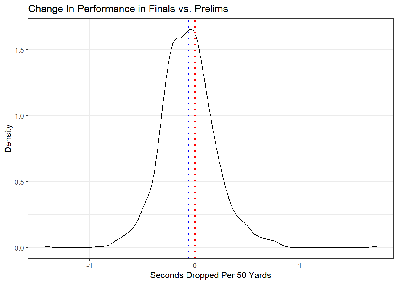
We can show this visually by plotting a density plot, with our sample mean denoted by a blue line, and our null hypothesis by a red one.
Drops %>%
  ggplot(aes(x = Per_Drop)) +
  geom_density() +
  geom_vline( # mean value
    aes(xintercept = mean(Per_Drop)),
    color = "blue",
    linetype = "dotted",
    size = 1
  ) +
  geom_vline( # null hypothesis at 0
    aes(xintercept = 0),
    color = "red",
    linetype = "dotted",
    size = 1
  ) +
  theme_bw() +
  labs(x = "Seconds Dropped Per 50 Yards",
       y = "Density",
       title = "Change In Performance in Finals vs. Prelims")
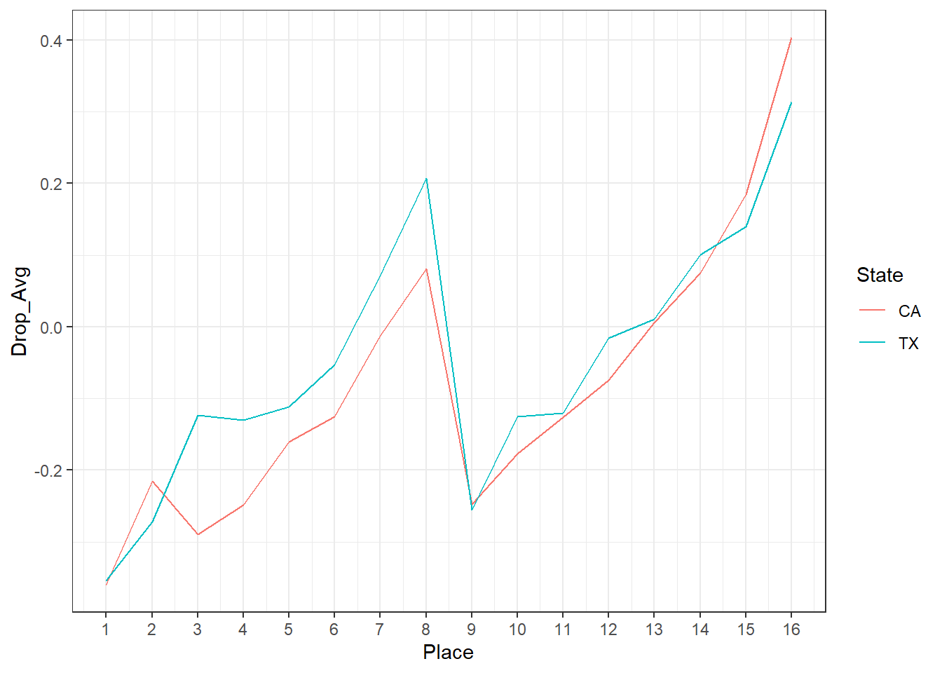
From the plot, and from the t.test results above, it’s clear that although swimmers do drop time, it’s not much time on average, only about 0.06 seconds. It might also be interesting to see how place impacts amount of time dropped. Let’s plot that.
Place_Drop <- Drops %>%
  group_by(Place, State) %>%
  summarise(Drop_Avg = mean(Per_Drop, na.rm = TRUE))

Place_Drop %>%
  ggplot() +
  geom_line(aes(x = Place, y = Drop_Avg, color = State)) +
  scale_x_continuous(breaks = seq(1, 16, 1)) +
  theme_bw()
There’s a couple things going on here. One is that the amount of time dropped tracks with place. Athletes who win tend to drop more time than those who come 16th. It could be that those athletes are just better, and “flip the switch” to deliver in the finals. It could also be that winning is lots of fun, and the chance to do so brings something more out of swimmers. Heck it could be both.
We can also see that there’s a big discontinuity around 8th-9th place. Those of you familiar with swimming can probably figure out what’s going on, and skip the rest of this paragraph where I’m going to explain it in excruciating detail. Assuming an 8 lane pool, which is the case for both the California and Texas meets, swimmers who place between 1st and 8th in the prelims swim in the “A” final at finals. These swimmers can place no higher than 1st (of course) and, critically, no lower than 8th overall long as they complete the race without being disqualified. That means that if a swimmer is in 8th place mid race and doesn’t think they can catch the 7th place swimmer there’s an incentive to just coast to the finish, because they’re guaranteed 8th regardless of their time. Similarly, swimmers who place between 9th and 16th in prelims swim in a “B” final at finals, where they can place no higher than 9th (regardless of time) and no lower than 16th. Getting 9th means winning the heat, and there’s a drive to do so. The further back one is in one’s heat though the more difficult it is to tell what’s going on, and be motivated to race those around you, and the less likely one is to win (the heat or the overall), so less drive to improve on a prelims time.
In Closing
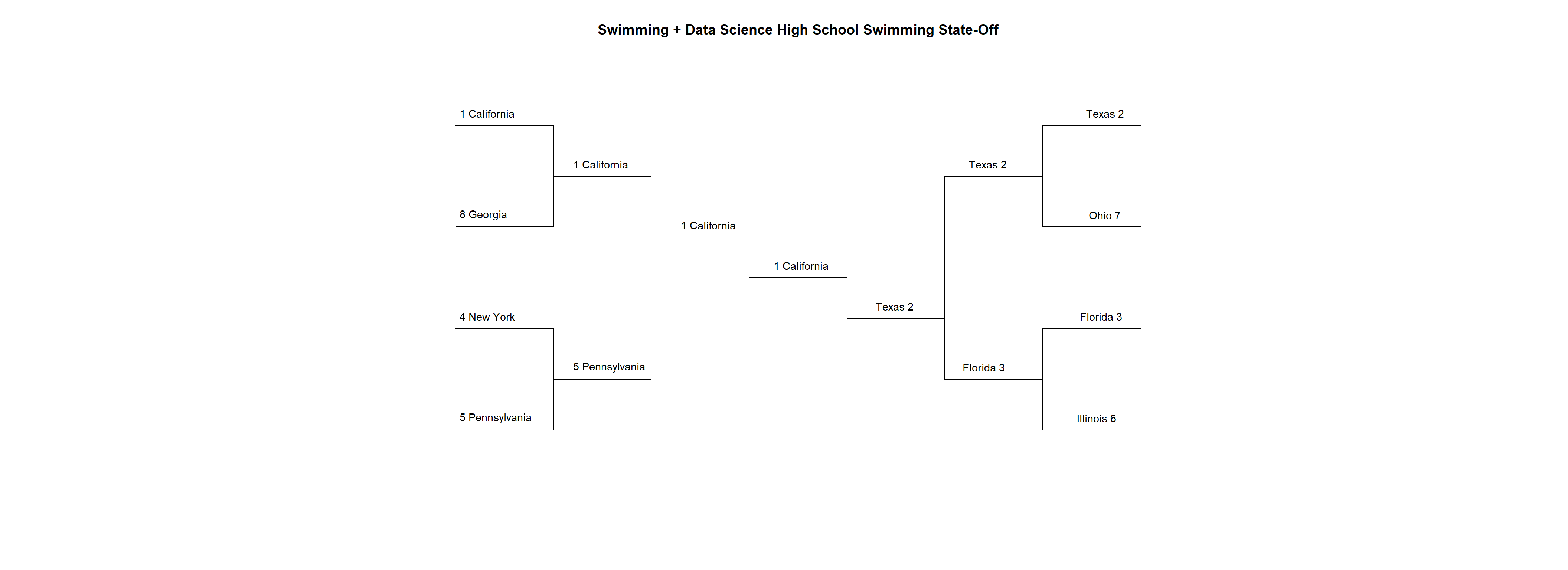
Well that’s it for the State-Off championship round. California, the number one seed, has in fact prevailed. There will be one more post in the State-Off series next week, where I’ll throw all 8 teams into one giant battle royale of a meet. Be sure to come back to Swimming + Data Science for that!
draw_bracket(
  teams = c(
    "California",
    "Texas",
    "Florida",
    "New York",
    "Pennsylvania",
    "Illinois",
    "Ohio",
    "Georgia"
  ),
  round_two = c("California", "Texas", "Florida", "Pennsylvania"),
  round_three = c("California", "Texas"),
  champion = "California",
  title = "Swimming + Data Science High School Swimming State-Off",
  text_size = 0.9
)
Updated: 17 November, 2021
Created: 17 September, 2020
